Probabilistic Grammars Research Paper

Most natural language processing systems are based on formal grammars. The development and study of formal grammars is known as computational linguistics. A grammar is a description of a language; usually it identifies the sentences of the language and provides descriptions of them, for example, by defining the phrases of a sentence, their interrelationships, and perhaps also aspects of their meanings. Parsing is the process of recovering a sentence’s description from its words, while generation is the process of translating a meaning or some other part of a sentence’s description into a grammatical or well-formed sentence. Parsing and generation are major research topics in their own right. Evidently, human use of language involves some kind of parsing and generation process, as do many natural language processing applications. For example, a machine translation program may parse an input language sentence into a (partial) representation of its meaning, and then generate an output language sentence from that representation.

Modern computational linguistics began with Chomsky (1957), and was initially dominated by the study of his ‘transformational’ grammars. These grammars involved two levels of analyses, a ‘deep structure’ meant to capture more-or-less simply the meaning of a sentence, and a ‘surface structure’ which reflects the actual way in which the sentence was constructed. The deep structure might be a clause in the active voice, ‘Sandy saw Sam,’ whereas the surface structure might involve the more complex passive voice, ‘Sam was seen by Sandy.’

Transformational grammars are computationally complex, and in the 1980s several linguists came to the conclusion that much simpler kinds of grammars could describe most syntactic phenomena, developing Generalized Phrase-Structure Grammars (Gazdar et al. 1985) and Unification-based Grammars (Kaplan and Bresnan 1982, Pollard and Sag 1987, Shieber 1986). These grammars generate surface structures directly; there is no separate deep structure and therefore no transformations. These kinds of grammars can provide very detailed syntactic and semantic analyses of sentences, but even today there are no comprehensive grammars of this kind that fully accommodate English or any other natural language.

Natural language processing using handcrafted grammars suffers from two major drawbacks. First, the syntactic coverage offered by any available grammar is incomplete, reflecting both our lack of understanding of even relatively frequently occuring syntactic constructions and the organizational difficulty of manually constructing any artifact as complex as a grammar of a natural language. Second, such grammars almost always permit a large number of spurious ambiguities, that is, parses which are permitted by the rules of syntax but have unusual or unlikely semantic interpretations. For example, in the sentence ‘I saw the boat with the telescope,’ the prepositional phrase ‘with the telescope’ is most easily interpreted as the instrument used in seeing, while in ‘I saw the policeman with the rifle,’ the prepositional phrase usually receives a different interpretation in which the policeman has the rifle. Note that the corresponding alternative interpretation is marginally accessible for each of these sentences: in the first sentence one can imagine that the telescope is on the boat, and in the second, that the rifle (say, with a viewing scope) was used to view the policeman.

In effect, there is a dilemma of coverage. A grammar rich enough to accommodate natural language, including rare and sometimes even ‘ungrammatical’ constructions, fails to distinguish natural from unnatural interpretations. But a grammar sufficiently restricted so as to exclude what is unnatural fails to accommodate the scope of real language. These observations led, in the 1980s, to a growing interest in stochastic approaches to natural language, particularly to speech. Stochastic grammars became the basis of speech recognition systems by outperforming the best of the systems based on deterministic handcrafted grammars. Largely inspired by these successes, computational linguists began applying stochastic approaches to other natural language processing applications. Usually, the architecture of such a stochastic model is specified manually, while the model’s parameters are estimated from a training corpus, that is, a large representative sample of sentences.

As explained in the body of this research paper, stochastic approaches replace the binary distinctions (grammatical vs. ungrammatical) of nonstochastic approaches with probability distributions. This provides a way of dealing with the two drawbacks of nonstochastic approaches. Ill-formed alternatives can be characterized as extremely low probability rather than ruled out as impossible, so even ungrammatical strings can be provided with an interpretation. Similarly, a stochastic model of possible interpretations of a sentence provides a method for distinguishing more plausible interpretations from less plausible ones.

The introduction sets out formally various classes of grammars and languages. Probabilistic grammars are introduced in Sect. 2, along with the basic issues of parametric representation, inference, and computation.

2. Grammars And Languages

The formal framework, whether used in a transformational grammar, a generalized phrase-structure grammar, or a more traditionally styled context-free grammar, is due to Chomsky (1957) and his co- workers. This section presents a brief introduction to this framework. But for a thorough (and very readable) presentation we highly recommend the book by Hopcroft and Ullman (1979).

The concept and notation of a formal grammar is perhaps best introduced by an example:

Example 1: Define a grammar, G₁, by G₁ = (T₁, N₁, S, R₁), where T₁ = {grows, rice, wheat} is a set of words (a ‘lexicon’), N₁ = {S, NP, VP} is a set of symbols representing grammatically meaningful strings of words, such as clauses or parts of speech (e.g., S for ‘Sentence,’ NP for ‘Noun Phrase,’ VP for ‘Verb Phrase’), and R₁ = {S → NP VP, NP → rice, NP → wheat, VP → grows} is a collection of rules for rewriting, or instantiating, the symbols in N₁. Informally, the nonterminal S rewrites to sentences or clauses, NP rewrites to noun phrases and VP rewrites to verb phrases. The language, L_G1, generated by G₁ is the set of strings of words that are reachable from S through the rewrite rules in R₁. In this example, L_G1 = rice grows, wheat grows , derived by S → NP VP → rice VP → rice grows, and S → NP VP → wheat VP → wheat grows.

More generally, if T is a finite set of symbols, let T * be the set of all strings (i.e., finite sequences) of symbols of T, including the empty string, and let T + be the set of all nonempty strings of symbols of T. A language is a subset of T *. A rewrite grammar G is a quadruple G = (T, N, S, R), where T and N are disjoint finite sets of symbols (called the terminal and nonterminal symbols respectively), SϵN is a distinguished nonterminal called the start or sentence symbol, and R is a finite set of productions. A production is a pair (α, β) where αϵN⁺ and β ϵ (N U T )*; productions are usually written α → β. Productions of the form α → ε, where ε is the empty string, are called epsilon productions. This entry restricts attention to grammars without epsilon productions, that is, β ϵ (N U T )⁺, as this simplifies the mathematics considerably.

A rewrite grammar G defines a rewriting relation →_G C (N U T )* × (N U T )* over pairs of strings consisting of terminals and nonterminals as follows: βAγ → βαγ iff A → α ϵ R and β, γ ϵ (N U T )* (the subscript G is dropped when clear from the context). The reflexive, transitive closure of → is denoted →*. Thus → * is the rewriting relation using arbitrary finite sequences of productions. (It is called ‘reflexive’ because the identity rewrite, α → α, is included.) The language generated by G, denoted L_G, is the set of all strings w ϵ T⁺ such that S → * w.

Rewrite grammars are traditionally classified by the shapes of their productions. G = (T, N, S, R) is a context-sensitive grammar if for all productions α → β ϵ R, |α| ≤ |β| , that is, the right-hand side of each production is not shorter than its left-hand side. G is a context-free grammar if |α| = 1, that is, the left-hand side of each production consists of a single non terminal. G is a left-linear grammar if G is context-free and β (the right-hand side of the production) is either of the form Aw or of the form w where A ϵ N and w ϵ T*; in a right-linear grammar β always is of the form wA or w. A right or left-linear grammar is called a regular grammar. G₁, in Example 1, is context sensitive and context free.

It is straightforward to show that the classes of languages generated by these classes of grammars stand in strict equality or subset relationships. Specifically, the class of languages generated by right-linear grammars is the same as the class generated by left-linear grammars; this class is called the regular languages, and is a strict subset of the class of languages generated by context-free grammars, which is a strict subset of the class of languages generated by context-sensitive grammars, which in turn is a strict subset of the class of languages generated by rewrite grammars.

It turns out that context-sensitive grammars (where a production rewrites more than one nonterminal) have not had many applications in natural language processing, so from here on we will concentrate on context-free grammars, where all productions take the form A → β, where A ϵ N and β ϵ (N U T )⁺.

An appealing property of grammars with productions in this form is that they induce tree structures on the strings that they generate. And, as Sect. 3 shows, this is the basis for bringing in probability distributions and the theory of inference. We say that the context-free grammar G = (T, N, S, R) generates the labeled, ordered tree ψ, iff the root node of ψ is labeled S, and for each node n in ψ, either n has no children and its label is a member of T (i.e., it is labelled with a terminal) or else there is a production A → β ϵ R where the label of n is A and the left-to-right sequence of labels of n’s immediate children is β. It is straightforward to show that w is in LG if G generates a tree ψ whose yield (i.e., the left-to-right sequence of terminal symbols labeling ψ’s leaf nodes) is w; ψ is called a parse tree of w (with respect to G). In what follows, we define Ψ_G to be the set of parse trees generated by G, and Y ( ) to be the function that maps trees to their yields.

Example 1 (continued): The grammar G₁ defined above generates the following two trees, ψ₁ and ψ₂.

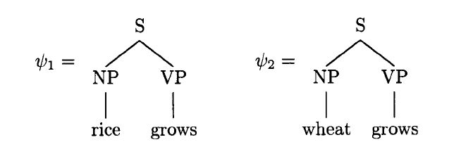
In this example, Y(ψ₁) = ‘rice grows’ and Y(ψ₂) = ‘wheat grows.’

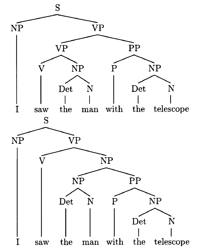
A string of terminals w is called ambiguous if w has two or more parse trees. Linguistically, each parse tree of an ambiguous string usually corresponds to a distinct interpretation.

Example 2: Consider G₂ = (T₂, N₂, S, R₂), where T₂ = {I, saw, the, man, with, telescope}, N₂ = {S, NP, N, Det, VP, V, PP, P} and R₂ = {S → NP, VP, NP → I, NP → Det N, Det → the, N → NP, PP, N → man, N → telescope, VP → V, NP, VP → VP, PP, PP → P, NP, V → saw, P → with . Informally, N rewrites to nouns, Det to determiners, V to verbs, P to prepositions and PP to prepositional phrases. It is easy to check that the two trees ψ₃ and ψ₄ with the yields Y(ψ₃) = Y(ψ₄) = ‘I saw the man with the telescope’ are both generated by G . Linguistically, these two parse trees represent two different syntactic analyses of the sentence. The first analysis corresponds to the interpretation where the seeing is by means of a telescope, while the second corresponds to the interpretation where the man has a telescope.

3. Probability And Statistics

Obviously broad coverage is desirable—natural language is rich and diverse, and not easily held to a small set of rules. But it is hard to achieve broad coverage without massive ambiguity (a sentence may have tens of thousands of parses), and this of course complicates applications like language interpretation, language translation, and speech recognition. This is the dilemma of coverage that we referred to earlier, and it sets up a compelling role for probabilistic and statistical methods.

We briefly review the main probabilistic grammars and their associated theories of inference. We begin in Sect. 3.1 with probabilistic regular grammars, also known as hidden Markov models (HMM), which are the foundation of modern speech recognition systems—see Jelinek (1997) for a survey.

In Sect. 3.2 we discuss probabilistic context-free grammars, which turn out to be essentially the same thing as branching processes. Finally, in Sect. 3.3, we take a more general approach to placing probabilities on grammars, which leads to Gibbs distributions, a role for Besag’s pseudolikelihood method (Besag 1974, 1975), various computational issues, and, all in all, an active area of research in computational linguistics.

3.1 Regular Grammars

We will focus on right-linear grammars, but the treatment of left-linear grammars is more or less identical. It is convenient to work with a normal form: all rules are either of the form A → bB or A → b, where A, B ϵ N and b ϵ T. It is easy to show that every right-linear grammar has an equivalent normal form in the sense that the two grammars produce the same language. Essentially nothing is lost.

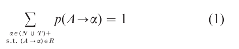
3.1.1 Probabilities. The grammar G can be made into a probabilistic grammar by assigning to each non terminal A ϵ N a probability distribution p over productions of the form A → α ϵ R: for every A ϵ N

Recall that Ψ_G is the set of parse trees generated by G (see Sect. 2). If G is linear, then ψ ϵ Ψ_G is characterized by a sequence of productions, starting from S. It is, then, straightforward to use p to define a probability P on Ψ_G: just take P (ψ) (for ψ ϵ Ψ_G) to be the product of the associated production probabilities.

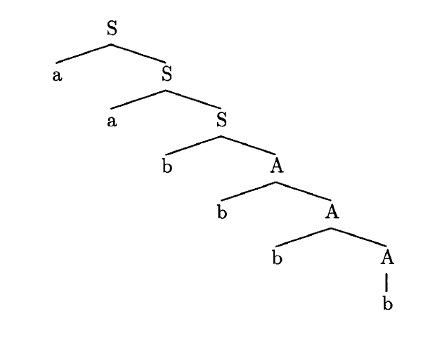
Example 3: Consider the right-linear grammar G₃ = (T₃, N₃, S, R₃), with T₃ = {a, b}, N₃ = {S, A} and the productions (R₃) and production probabilities ( p):

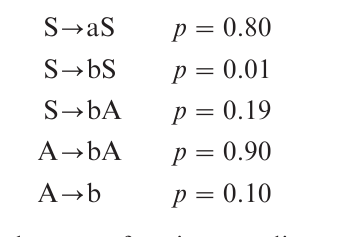
The language is the set of strings ending with a sequence of at least two bs. The grammar is ambiguous: in general, a sequence of terminal states does not uniquely identify a sequence of productions. The sentence aabbbb has three parses (determined by the placement of the production S → bA), but the most likely parse, by far, is S → aS, S → aS, S → bA, A → bA, A → bA, A → b (P = 0.8 • 0.8 • 0.19 • 0.9 • 0.1), which has a posterior probability of nearly 0.99. The corresponding parse tree is shown below.

3.1.2 Inference. The problem is to estimate the transition probabilities, p(•), either from parsed data (examples from Ψ_G) or just from sentences (examples from L_G). Consider first the case of parsed data (‘supervised learning’), and let ψ₁, ψ₂,…, ψ_n ϵ Ψ be a sequence taken iid according to P. If f(A → α; ψ) is the counting function, counting the number of times transition A → α ϵ R occurs in ψ, then the likelihood function is

The maximum likelihood estimate is, sensibly, the relative frequency estimator:

The problem of estimating p from sentences (‘unsupervised learning’) is more interesting, and more important for applications. Recall that Y (ψ) is the yield of ψ, that is. the sequence of terminals in ψ. Given a sentence w ϵ T⁺, let Ψ_w be the set of parses which yield w: Ψ_w = {ψ ϵ Ψ: Y(ψ) = w}. Imagine a sequence ψ₁,… ,ψ_n, iid according to P, for which only the corresponding yields, w_i = Y(ψ_i) 1 ≤ i ≤ n, are observed. The likelihood function is

As is usual with hidden data, there is an EM-type iteration for climbing the likelihood surface—see Baum (1972) and Dempster et al. (1977):

Needless to say, nothing can be done with this unless we can actually evaluate, in a computationally feasible way, expressions like E_p[ f(A → α; ψ)|ψ ϵ Ψ_w]. This is one of several closely related computational problems that are part of the mechanics of working with regular grammars.

3.1.3 Computation. A sentence w ϵ T⁺ is parsed by finding a sequence of productions A → bB ϵ R which yield w. Depending on the grammar, this corresponds more or less to an interpretation of w. Often, there are many parses and we say that w is ambiguous. In such cases, if there is a probability p on R then there is a probability P on Ψ, and a reasonably compelling choice of parse is the most likely parse:

This is the maximum a posteriori (MAP) estimate of ψ—obviously it minimizes the probability of error under the distribution P. (Of course, in those cases in which Eqn. (6) is small, P does little to make w unambiguous.)

What is the probability of w? How are its parses computed? How is the most likely parse computed? These computational issues turn out to be more-or-less the same as the issue of computing E_p [ f (A →α; ψ) ψ ϵ Ψ_w] that came up in our discussion of inference. The basic structure and cost of the computational algorithm is the same for each of the four problems— compute the probability of w, compute the set of parses, compute the best parse, compute Ep. In particular, there is a simple dynamic programming solution to each of these problems, and in each case the complexity is of the order n•|R|, where n is the length of w, and R is the number of productions in G—see Jelinek (1997), Geman and Johnson (2000). The existence of a dynamic programming principle for regular grammars is a primary reason for their central role in state-of-the-art speech recognition systems.

3.2 Context-Free Grammars

Despite the successes of regular grammars in speech recognition, the problems of language understanding and translation are generally better addressed with the more structured and more powerful context-free grammars. Following our development of probabilistic regular grammars in the previous section, we will address here the interrelated issues of fitting contextfree grammars with probability distributions, estimating the parameters of these distributions, and computing various functionals of these distributions.

The context-free grammars G = (T, N, S, R) have rules of the form A → α, α ϵ (N U T )⁺, as discussed previously in Sect. 2. There is again a normal form, known as the Chomsky normal form, which is particularly convenient when developing probabilistic versions. Specifically, one can always find a context free grammar G´, with all productions of the form A → BC or A → a, A , B, C ϵ N, α ϵ T, which produces the same language as G: L_G = L_G. Henceforth, we will assume that context-free grammars are in the Chomsky normal form.

3.2.1 Probabilities. The goal is to put a probability distribution on the set of parse trees generated by a context-free grammar in Chomsky normal form. Ideally, the distribution will have a convenient parametric form, that allows for efficient inference and computation.

Recall from Sect. 2 that context-free grammars generate labeled, ordered trees. Given sets of nonterminals N and terminals T, let Ψ be the set of finite trees with:

(a) root node labeled S;

(b) leaf nodes labeled with elements of T;

(c) interior nodes labeled with elements of N;

(d) every nonterminal (interior) node having eithertwo children labeled with nonterminals or one child labeled with a terminal.

Every ψ ϵ Ψ defines a sentence w ϵ T⁺: read the labels off of the terminal nodes of ψ from left to right. Consistent with the notation of Sect. 3.1 we write Y(ψ) = w. Conversely, every sentence w ϵ T⁺ defines a subset of Ψ, which we denote by Ψ_w, consisting of all ψ with yield w (Y(ψ) = w). A context-free grammar G defines a subset of Ψ, Ψ_G, whose collection of yields is the language, L_G, of G. We seek a probability distribution P on Ψ which concentrates on Ψ_G.

The time-honored approach to probabilistic context-free grammars is through the production probabilities p : R → [0, 1], with

Following the development in Sect. 3.1, we introduce a counting function f (A → α; ψ), which counts the number of instances of the rule A → a in the tree ψ, i.e., the number of nonterminal nodes A whose daughter nodes define, left-to-right, the string α. Through f, p induces a probability P on Ψ:

It is clear enough that P concentrates on ΨG, and we shall see shortly that this parameterization, in terms of products of probabilities p, is particularly workable and convenient. The pair, G and P, is known as a probabilistic context-free grammar, or PCFG for short. (Notice the connection to branching processes—Harris (1963): Starting at S, use R, and the associated probabilities p( ), to expand nodes into daughter nodes until all leaf nodes are labeled with terminals—i.e., with elements of T.)

3.2.2 Inference. As with probabilistic regular grammars, the production probabilities of a context-free grammar, which amount to a parameterization of the distribution P on Ψ_G, can be estimated from examples. In one scenario, we have access to a sequence ψ₁, …, ψ_n from Ψ_G under P. This is ‘supervised learning,’ in the sense that sentences come equipped with parses. More practical is the problem of ‘unsupervised learning,’ wherein we observe only the yields, Y(ψ₁), …, Y(ψ_n).

In either case, the treatment of maximum likelihood estimation is essentially identical to the treatment for regular grammars. In particular, the likelihood for fully observed data is again Eqn. (2), and the maximum likelihood estimator is again the relative frequency estimator Eqn. (3). And, in the unsupervised case, the likelihood is again Eqn. (4) and this leads to the same EM-type iteration given in Eqn. (5).

3.2.3 Computation. There are again four basic computations: find the probability of a sentence w ϵ T⁺, find a ψ ϵ Ψ (or find all ψ ϵ Ψ) satisfying Y(ψ) = w (‘parsing’); find

(‘maximum a posteriori’ or ‘optimal’ parsing); compute expectations of the form E_pt[ f (A → α; ψ)|ψ ϵ Ψ_w] that arise in iterative estimation schemes like (5). The four computations turn out to be more-or-less the same, as was the case for regular grammars (Sect. 3.1.3) and there is again a common dynamic- programming-like solution—see Lari and Young (1990, 1991), Geman and Johnson (2000).

3.3 Gibbs Distributions

There are many ways to generalize. The coverage of a context-free grammar may be inadequate, and we may hope, therefore, to find a workable scheme for placing probabilities on context-sensitive grammars, or perhaps even more general grammars. Or, it may be preferable to maintain the structure of a context-free grammar, especially because of its dynamic programming principle, and instead generalize the class of probability distributions away from those induced (parameterized) by production probabilities. But nothing comes for free. Most efforts to generalize run into nearly intractable computational problems when it comes time to parse or to estimate parameters.

Many computational linguists have experimented with using Gibbs distributions, popular in statistical physics, to go beyond production-based probabilities, while nevertheless preserving the basic context-free structure. Next we take a brief look at this particular formulation, in order to illustrate the various challenges that accompany efforts to generalize the more standard probabilistic grammars.

3.3.1 Probabilities. The sample space is Ψ_G, the set of trees generated by a context-free grammar G. Gibbs measures are built from sums of more-or-less simple functions, known as ‘potentials’ in statistical physics, defined on the sample space. In linguistics, it is more natural to call these features rather than potentials. Suppose, then, that we have identified M linguistically salient features f₁, …, f_M, where f_k: Ψ_G → R, through which we will characterize the fitness or appropriateness of a structure ψ ϵ Ψ_G. More specifically, we will construct a class of probabilities on Ψ_G which depend on ψ ϵ Ψ_G only through f₁(ψ), …, f_M(ψ). Examples of features are the number of times a particular production occurs, the number of words in the yield, various measures of subjectverb agreement, and the number of embedded or independent clauses.

Gibbs distributions have the form

where θ₁, …, θ_M are parameters, to be adjusted ‘by hand’ or inferred from data, θ = (θ₁, …, θ_M), and where Z = Z(θ) (known as the ‘partition function’) normalizes so that P_θ(Ψ) = 1. Evidently, we need to assume or ensure that ∑_ψcΨGexp {∑^M₁θ_i f_i(ψ)} < ∞. For instance, we had better require that θ₁ < 0 if M = 1 and f₁(ψ) =|Y(ψ)| (the number of words in a sentence), unless of course |Ψ_G | < ∞.

3.3.2 Relation To Probabilistic Context-Free Grammars. Gibbs distributions are much more general than probabilistic context-free grammars. In order to recover PCFG’s, consider the special feature set {f (A → α; ψ)}_{A → αϵR}: The Gibbs distribution Eqn. (9) takes on the form

Evidently, then, we get the probabilistic context-free grammars by taking θ_A→α = log_ep(A → α), where p is a system of production probabilities consistent with Eqn. (7), in which case Z = 1. But is Eqn. (10) more general? Are there probabilities on Ψ_G of this form that are not PCFGs? The answer turns out to be no, as was shown by Chi (1999) and Abney et al. (1999): given a probability distribution P on Ψ_G of the form of Eqn. (10), there always exists a system of production probabilities p under which P is a PCFG.

3.3.3 Inference. The feature set {f_i}_{i= 1,…,M} can be accommodate arbitrary linguistic attributes and constraints, and the Gibbs model Eqn. (9), therefore, has great promise as an accurate measure of linguistic fitness. But the model depends critically on the parameters {θ_i}_{i = 1,…,M}, and the associated estimation problem is, unfortunately, very hard. Indeed, the problem of unsupervised learning appears to be all but intractable.

Let us suppose, then, that we observe ψ₁, ψ₂, …,ψ_n ϵ Ψ _G (‘supervised learning’), iid according to P_θ. In general, the likelihood function, Пⁿ_i=1P_θ (ψ_i), is more or less impossible to maximize. But if the primary goal is to select good parses, then perhaps the likelihood function asks for too much, or even the wrong thing. It might be more relevant to maximize the likelihood of the observed parses, given the yields Y(ψ₁),…, Y(ψ_n):

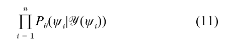
Maximization of Eqn. (11) is an instance of Besag’s remarkably effective pseudo likelihood method (Besag 1974, 1975), which is commonly used for estimating parameters of Gibbs’s distributions. The computations involved are generally much easier than what is involved in maximizing the ordinary likelihood function. Take a look at the gradient of the logarithm of Eqn. (11): the θ_j component is proportional to

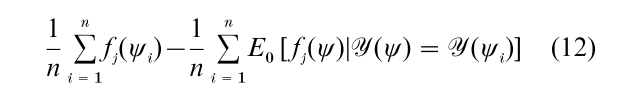
and E_θ[ f_j(ψ)|Y(ψ)] can be computed directly from the set of parses of the sentence Y(ψ). (In practice there is often massive ambiguity, and the number of parses may be too large to feasibly consider. Such cases require some form of pruning or approximation.)

Thus gradient ascent of the pseudolikelihood function is (at least approximately) computationally feasible. This is particularly useful since the Hessian of the logarithm of the pseudolikelihood function is nonpositive, and therefore there are no local maxima. What is more, under mild conditions pseudolikelihood estimators (i.e., maximizers of Eqn. (11)) are consistent; (Chi 1998).

Bibliography:

1. Abney S, McAllester D, Pereira F 1999 Relating probabilistic grammars and automata. In: Proceedings of the 37th Annual Meeting of the Association for Computational Linguistics, Morgan Kaufmann, San Francisco, pp. 542–609
2. Baum L E 1972 An inequality and associated maximization techniques in statistical estimation of probabilistic functions of Markov processes. Inequalities 3: 1–8
3. Besag J 1974 Spatial interaction and the statistical analysis of lattice systems (with discussion). Journal of the Royal Statistical Society, Series D 36: 192–236
4. Besag J 1975 Statistical analysis of non-lattice data. The Statistician 24: 179–95
5. Chi Z 1998 Probability models for complex systems. PhD thesis, Brown University
6. Chi Z 1999 Statistical properties of probabilistic context-free grammars. Computational Linguistics 25(1): 131–60
7. Chomsky N 1957 Syntactic Structures. Mouton, The Hague
8. Dempster A, Laird N, Rubin D 1977 Maximum likelihood from incomplete data via the EM algorithm. Journal of the Royal Statistical Society, Series B 39: 1–38
9. Fu K S 1974 Syntactic Methods in Pattern Recognition. Academic Press, New York
10. Fu K S 1982 Syntatic Pattern Recognition and Applications. Prentice-Hall, Englewood Cliffs, NJ
11. Gazdar C, Klein E, Pullum G, Sag I 1985 Generalized Phrase Structure Grammar. Blackwell, Oxford, UK
12. Geman S, Johnson M 2000 Probability and statistics in computational linguistics, a brief review. Internal publication, Division of Applied Mathematics, Brown University
13. Harris T E 1963 The Theory of Branching Processes. Springer, Berlin
14. Hopcroft J E, Ullman J D 1979 Introduction to Automata Theory, Languages and Computation. Addison-Wesley, Reading, MA
15. Jelinek F 1997 Statistical Methods for Speech Recognition. MIT Press, Cambridge, MA
16. Kaplan R M, Bresnan J 1982 Lexical functional grammar: A formal system for grammatical representation. In: Bresnan J (ed.) The Mental Representation of Grammatical Relations. MIT Press, Cambridge, MA, Chap. 4, pp. 173–281
17. Kay M, Gawron J M, Norvig P 1994 Verbmobil: A Translation System for Face-to-face Dialog. CSLI Press, Stanford, CA
18. Lari K, Young S J 1990 The estimation of stochastic context-free grammars using the inside-outside algorithm. Computer Speech and Language 4: 35–56
19. Lari K, Young S J 1991 Applications of stochastic context-free grammars using the inside-outside algorithm. Computer Speech and Language 5: 237–57
20. Pollard C, Sag A 1987 Information-based Syntax and Semantics. CSLI Lecture Notes Series No.13. University of California Press, Stanford, CA
21. Shieber S M 1986 An Introduction to Unification-based Approaches to Grammar. CSLI Lecture Notes Series. University of California Press, Stanford, CA