Inverse Projection Research Paper

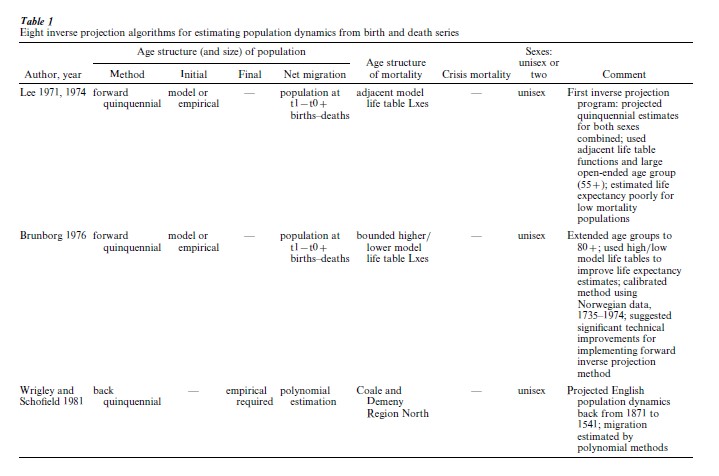
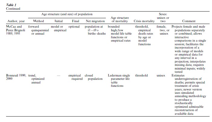
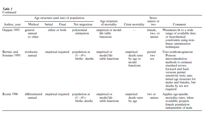
Surprisingly accurate demographic statistics can be computed with the inverse projection method. As with most demographic techniques, the better the data, the better the estimates. What is startling about inverse projection is how little data is required to simulate the demographic history of places, large and small, over long periods of time within a range of a few percentage points (Lee 1985, McCaa 1989, McCaa and Vaupel 1992). Recent innovations (see Table 1) fine-tune the method to offer several different algorithms, including a stochastic microsimulation process which estimates not only a wide range of age-dependent demographic rates and measures but most importantly their standard errors (Bertino and Sonnino 1995).

Inverse projection is a method for estimating basic demographic statistics where the vital or parish registration system is relatively efficient, but where population censuses or surveys are lacking, infrequent, or unreliable. The technique requires a count of births and deaths year by year, and the size of the initial population. In the absence of reliable empirical age data, model age structures of mortality, fertility, migration, and even the initial population may be relied upon. In contrast to family reconstitution, inverse projection requires only aggregate data of births and deaths, tallied by year. Thus, the demo-graphic history of large areas is easily reconstructed with inverse methods. Where family reconstitution is labor intensive, inverse projection demands little effort to tally and computerize annual counts of births and deaths. Finally, family reconstitution’s stringent methodological rules exclude a sizeable fraction of births and deaths from the calculations. The reconstitutable minority is unlikely to be representative of the majority of the population. Inverse projection applies powerful nonlinear models to data for the entire population. It is superior to stable population methods because no assumption of stability is required.

The inverse method has been used to construct population histories of states (England 1541–1871, Norway 1735–1974, Sweden 1750–1875, Denmark, the Philippines, Valencia 1610–1899, Italy 1750–1911, Chile 1855–1964, Bulgaria, Costa Rica, and Cuba 1900–59), regions (Northern Italy 1650–1881, the Canary Islands 1680–1850, Sardinia 1862–1921, and Scania 1650–1760), cities, parishes, and even missions (Colyton 1545–1834, Pays de Caux 1530–1700, Lucerne 1700–1930, Berne 1720–1920, Amsterdam 1680–1921, Velletri 1595–1740, and California). This list, although incomplete, includes studies which test a wide range of demographic hypotheses, from models of population change in industrializing Europe to demographic responses to epidemics.

2. History And Scope

Since Lee first created inverse projection in 1971, seven additional implementations of the method have been developed (Table 1). In each case, macrodemographic data for a parish, city, region, nation, or other geographical or administrative unit are required. The algorithms differ in the use of models to supplement missing or unknown parameters. In recent decades, as computing power increased, so has the sophistication and computational demands of the various methods.

Lee’s classic forward inverse algorithm (1974) re-mains the simplest and most straightforward. Total population is required to initiate the projection. Counts of births for each period (quinquennia in Lee’s first program) are added and deaths subtracted to obtain the population at the end of each interval. Where a count of the total population is known for a subsequent period, the projected total is subtracted from the observed to obtain an estimate of net migration, which is apportioned equally among the intervening periods.

The initial age structure of the population may be obtained from either a census or a model. Lacking an empirically derived age structure, the demographically naive might stop at this point, but Lee (1974, 1985) and others have shown that even an arbitrarily chosen model age structure yields remarkably robust estimates (Brunborg 1976, Wachter 1986, McCaa 1989, McCaa and Vaupel 1992, McCaa 1993). Moreover, the bias of a poor choice rapidly disappears as the stream of vital rates molds the projected age structure period by period with births added to the base of the pyramid at age zero and deaths subtracted from the slope, age by age.

‘Vital rates, not initial states’ is the inverse projectionist’s mantra, but this is not a matter of faith. The theoretical foundations of inverse projection lie in the 1920s with the work of H. T. J. Norton on the weak ergodicity theorem, and in the 1960s with its re- discovery by Alvaro Lopez (Wachter 1986). The method rests on what Kenneth Wachter has called ‘the cornerstone of formal demography’: the notion that, in the long run, vital rates, not initial states, determine what a population will look like. Lee has shown that population age structures are quickly forgotten, even when punctuated by demographically critical events such as epidemics, wars, baby booms, and baby busts (Lee 1985). The weak ergodicity theorem teaches that when it comes to age distributions, populations have no memory. As populations are projected through time, the initial age structure is displaced by consequences of birth, death, and migration rates. For all practical purposes, populations subject to the same initial population size and identical streams of births, deaths, and migration will converge, even though they may begin from radically different age structures. A century into a projection erases even the most peculiar initial age structure. On the other hand, population size remains a powerful constraint. If it is misspecified and the population growth rate is negative, distortions will mushroom. Where the population is growing, the effect of this bias diminishes over time (McCaa and Vaupel 1992).

The ingenuity of Lee’s method is how, in the absence of data, deaths are apportioned by age (Lee 1974). As a first approximation, an arbitrary set of age-specific death rates from a single-parameter family of life tables is applied for the quinquennium. The product of these rates and the age structure at the beginning of the interval yields an estimate of the number of deaths for each age group. Adding over all groups and dividing by the total number of observed deaths yield an adjustment factor called the normalized death ratio. This factor is a measure of the discrepancy between the observed number of deaths and the number projected given the age structure and level of mortality from model life-table rates. As a second and final approximation, the normalized death ratio is used to compute the exact number of deaths at each age. These numbers will add up to the total fror the entire interval. This is accomplished directly by, first, subtracting age-specific rates between the model life table used in step 1 and an adjacent table from the same family. The result is a domain of mortality variability at each age. This domain is used to interpolate an adjusted age-specific death rate. This is accomplished by multiplying the normalized death ratio and the mortality domain at each age and adding the result to the first approximation. This yields a final estimate of deaths for each age group. Added up, they equal the total deaths for the period. Net migration by age is apportioned crudely as a function of age-specific rates and a level parameter for each period. Where migration is minor relative to mortality, this solution—required due to lack of data—produces acceptable results. Fertility statistics are by-products of inverse projection, and are wholly independent of age estimation and projection. The number of births for each time interval is determined by the stream of vital events. What is lacking is a summary fertility statistic which takes into account the age structure of the population. A solution common to all inverse projection algorithms is the estimation of the gross reproduction ratio from the number of births, the age structure of the population, and a normalized age pattern of fertility.

3. Expansions

Four important expansions of Lee’s inverse method emerged in the last decades of the twentieth century: a full range of age groups, annual projections, crisis mortality, and two-sex models. To reduce computation costs, Lee’s 1971 algorithm crudely lumped the oldest ages into a group for ages 55 and over. Extending the number of age groups beyond age 55 and over so that the final, open-ended group accounts for only a small fraction of total deaths was the first, most significant, and least controversial innovation in inverse projection methods. Brunborg (1976) quickly discovered that this shortcut introduces a substantial bias, particularly where a large fraction of total deaths occurs in the final age group. As long as life expectancy at birth is less than 30 years, the effect of lumping is small, but where life expectancy is moderately good, highly variable, or improving, error becomes substantial. Brunborg’s algorithm and all subsequent ones allow the user to apply a more reasonable upper-age interval, such as 75, 90, or even 100 years and older.

A second important enhancement of the inverse method was the development of single-year projections in place of five- or 10-year periods. Anticipated by Lee and Brunborg, annual projection cycles were first implemented by Bonneuil’s trend method (1993). Initially, there were objections to annual projections as spurious precision until Bonneuil demonstrated that aggregation into five-or 10-year periods can introduce serious distortions. Aggregation flattens mortality variation, and thereby flattens the population age structure whenever a mortality crisis occurs. With quinquennial or decennial projections, mortality domain interpolation dampens variation throughout the population age structure. Annual mortality spikes are transformed, at best, into waves which continue to undulate through the age pyramid over subsequent cycles. Now that computation costs are no longer a constraint, annual projections are becoming common, although some inverse projection algorithms still permit quinquennial or even decennial projections as an option. Crisis mortality, due (say) to epidemics, famine, or other demographic catastrophes, is poorly approximated by model life tables. For the inverse projectionist, the alternative is either to apply a special set of age-specific death rates (empirical or model) for the crisis years (Bertino and Sonnino 1995) or to fix a crude death-rate threshold to mimic the impact of crises on the population age structure (Bonneuil 1993, McCaa 1993). In crisis years, mortality domain interpolation will assign too many deaths to age groups in which the spread is greatest, principally to infants, children, and the oldest or open-ended age group. The optimal solution is to use empirically derived age-specific death rates peculiar to the type of crisis. Less desirable, although widely used due to the scarcity of age-specific data for these situations, is to set a mortality threshold, say a crude death rate of 40 per thousand population (Bonneuil 1993, McCaa and Vaupel 1992, McCaa 1993). Deaths below the threshold are apportioned according to standard inverse methodology. Any excess is then apportioned at a flat rate for each age group. Although this is an arbitrary fix, the effect is to produce more robust estimates of life expectancy and population age structure than that provided by the standard method.

Single-sex projections were the norm with the first inverse projection programs, produced when computer time was scarce. Now that this is no longer a constraint, two-sex projections are becoming frequent where births, deaths, and population size are readily available by sex. Precision is an obvious benefit, and so is the ability to model gender differences in mortality and migration.

4. Related Methods

Back projection was developed as a means of dealing with the closure problem. Wrigley and Schofield used back inverse projection for their massive reconstruction of the population of England, 1541–1871 (Wrigley and Schofield 1981, Oeppen 1993b). In the long run, most populations are not closed, and that of England is no exception. While forward inverse projection takes into account authentic migration data, Lee’s method cannot produce migration flows (Lee 1993). Back projection seeks to generate migration estimates from a terminal age structure by back casting the population against the flow of births and deaths. While it might seem commonsensical to begin with the best, i.e., most recent, data and project backward, Lee argues that this ignores the weak ergodicity theorem. In Lee’s words (1993), ‘the problem originates with the attempt to resurrect people who have died into the oldest age group, an attempt that is, in practice, hypersensitive to error.’ The Cambridge team used iteration procedures to settle upon a single series of best estimates.

Generalized inverse projection is a response to Lee’s criticisms of back projection, and broadens the method into an analytical system which exploits whatever data are available as well as a broad range of assumptions or constraints, including components derived from back projection (Oeppen 1993a, 1993b). Generalized inverse projection uses a standard method of demographic accounting and standard nonlinear optimization algorithm to overcome a range of empirical and theoretical problems. Among these is the temptation to estimate migration endogenously by means of smoothing parameters.

Other flavors of inverse projection were developed, on the one hand, to extend projections back to the first years of parish registration, where either the birth or death series begins somewhat earlier than the other (Bonneuil 1993, 2000), and, on the other, to maximize the use of data available in specific countries, such as population censuses or status animarum containing age details (Rosini1996). The most innovative recent algorithm is stochastic inverse projection, a micro-simulation technique which seeks to assess the variability in a population’s evolution (Bertino and Sonnino 1995). Instead of a single deterministic solution as with forward inverse projection, the stochastic method offers many solutions by simulating individual mortality events as a nonhomogeneous Poisson process. Three additional assumptions are required: deaths must be uniformly distributed over the year, they must be independent of each other, and every person must have the same mortality function as contemporaries at each point in time.

5. Calibration And Limitations

Lee first calibrated the method against family reconstitution results for the parish of Colyton, 1545–1834 (Lee 1974). In addition to confirming the general findings of an excellent family reconstitution study of Colyton, Lee was able to gain new insight on periodic shifts in fertility and mortality that are not readily discernible with the family reconstitution method. For example, he placed life expectancy at birth for the plague years 1645–9 at less than nine years. A second important calibration was Brunborg’s reconstruction of the population history of Norway, which he compared with statistics derived from highly accurate age-specific data over the course of more than a century (Brunborg 1976). The results were remarkably consistent, tracking the official life expectancy at birth figures from a low of 43.7 years in the 1830s to a high of 74 years in the late 1960s. Average error was roughly two years. What most surprised Brunborg was how little difference the various mortality suppositions made on the estimates of life expectancy and age structure.

The most important lesson from Brunborg’s experiments was that the quality of data is the critical factor for successful inverse projections. Later his findings were confirmed by a series of wide-ranging tests by a skeptical demographer, who challenged an inverse projection enthusiast to a double-blind experiment, indeed to a dozen such experiments (McCaa and Vaupel 1992). Vaupel used conventional cohort component projection techniques to simulate a wide range of demographic histories and challenged McCaa to reproduce the results for each from the bare minimum required for inverse projection: the birth and death series, and initial population size. The results were spectacularly successful; so much so that they led to the discovery of a flaw (bug) in the benchmarking program.

Vaupel’s challenge led to the discovery that the required model age data could be ascertained directly by minimizing the normalized mortality ratio. This statistic can be used as a measure of goodness of fit where model age data are required, such as for the initial population and the age structure of mortality (McCaa 1993). The k ratio is an indicator of the age-standardized intensity of mortality relative to the initial age structure of the population and to the pair of age-specific mortality schedules used to project the population by age to the next period. The sum of squares of this ratio is a useful measure of goodness of fit when the birth and death series and initial population size are held constant. In other words, where two inverse projections differ only in terms of model age structures of mortality or initial population, the squared ratio can be used to identify the better-fitting models. Best-fitting models have the lowest squared ratios. However, if the statistic is to be a reliable guide, the stream of counts and initial population size must remain the same to compare projection results.

Vaupel’s challenge confirmed that data quality remains the most important constraint for successfully applying the method. Careful attention should be given to spikes in mortality or surges in migration. They may confound the normality assumption of how these events should be distributed over the age structure.

6. Prospects

The inverse method requires good vital registration data. For historical studies, this limits its usefulness primarily to the European cultural area. Nevertheless, even here, only a small number of potential applications have been attempted. Lee’s challenge that the method be extended to the modeling of marriage and legitimate fertility has gone unanswered. The inverse method could also be extended to other demographic measures where authentic scale parameters are avail-able and age patterns can be modeled, as in the case of parity progression ratios (Feeney 1985). The most important contribution of the method is its illumination of demographic processes in the past. In the case of England, for example, thanks to inverse projection we now know that the great surge of population in the late eighteenth century was due to a rise in fertility, rather than to a fall in mortality, as had long been supposed (Wrigley and Schofield 1981).

Bibliography:

1. Bertino S, Sonnino E 1995 La proiezione inversa stocastica: Tecnicave applicazione. Le Italie Demografiche. Saggi di demografia storica. University of Udine, Rome
2. Biraben J N, Bonneuil N 1986 Population et Societe en Pays de Caux au XVIIe siecle. Population 6: 937–60
3. Bonneuil N 1993 The trend method applied to English data. In: Reher D S, Schofield R (eds.) Old and New Methods in Historical Demography. Clarendon Press, Oxford, UK, pp. 57–65
4. Brunborg H 1976 The inverse projection method applied to Norway, 1735–1974. Unpublished ms.
5. Feeney G 1985 Parity progression projection. In: International Population Conference, Florence 1985. International Union for the Scientific Study of Population, Vol. 4, pp. 125–36
6. Galloway P R 1994 A reconstruction of the population of north Italy from 1650 to 1881 using annual inverse projection with comparisons to England, France, and Sweden. European Journal of Population Revue Europeenne de Demographie 10: 223–74
7. Lee R D 1974 Estimating series of vital rates and age structures from baptisms and burials: A new technique with applications to pre-industrial England. Population Studies 28: 495–512
8. Lee R D 1985 Inverse projection and back projection: A critical appraisal and comparative results for for England, 1539–1871. Population Studies 39: 233–48
9. Lee R D 1993 Inverse projection and demographic fluctuations: a critical assessment of new methods. In: Reher D S, Schofield R (eds.) Old and New Methods in Historical Demography. Clarendon Press, Oxford, UK, pp. 7–28
10. Leeuwenn M H D, Oppen J 1993 Reconstructing the demo-graphic regime of Amsterdam 1681–1920. Economic and Social History in The Netherlands 5: 61–102
11. McCaa R 1989 Populate: A microcomputer projection package for aggregative data applied to Norway, 1736–1970. Annales de Demographie Historique. 287–298
12. McCaa R 1993 Benchmarks for a new inverse population projection program: England, Sweden, and a standard demo-graphic transition. In: Reher D S, Schofield R (eds.) Old and New Methods in Historical Demography. Clarendon Press, Oxford, UK, pp. 40–56
13. McCaa R, Perez Brignoli H 1989 Populate: From Births and Deaths to the Demography of the Past, Present, and Future. University of Minnesota, Minneapolis, MN
14. McCaa R, Vaupel J W 1992 Comment la projection inverse se comporte-t-elle sur des donnees simulees. In: Blum A, Bonneuil N, Blanchet D (eds.) Modeles de la demographie historique. National Institute for the Study of Demographics, Paris, pp. 129–46
15. Oeppen J 1993a Back projection and inverse projection: Members of a wider class of constrained projection models. Population Studies 47: 245–67
16. Oeppen J 1993b Generalized inverse projection. In: Reher D S, Schofield R (eds.) Old and New Methods in Historical Demography. Clarendon Press, Oxford, UK, pp. 29–39
17. Rosina A 1996 IPD 3.0: Aplicazione automatica dell’in erse projection differenziata (passo annualeve quinquennale). University of Padua, Padua, Italy
18. Wachter K W 1986 Ergodicity and inverse projection. Population Studies 40: 275–87
19. Wrigley E A, Davies R S, Oeppen J, Schofield R S 1997 Reconstitution and inverse projection. In: English Population History from Parish Reconstitutions, Cambridge University Press, Cambridge, UK
20. Wrigley E A, Schofield R S 1981 The Population History of England, 1541–1871: A Reconstruction. Harvard University Press, Cambridge, MA