Demographic Measurement Research Paper

Let us now consider some further types of demographic behavior.

1. Marriage, Cohabitation, And Union Disruption Divorce

Measures of marriage and divorce are much less numerous than are those of fertility. We consider them under the headings of level and timing.

1.1 Level

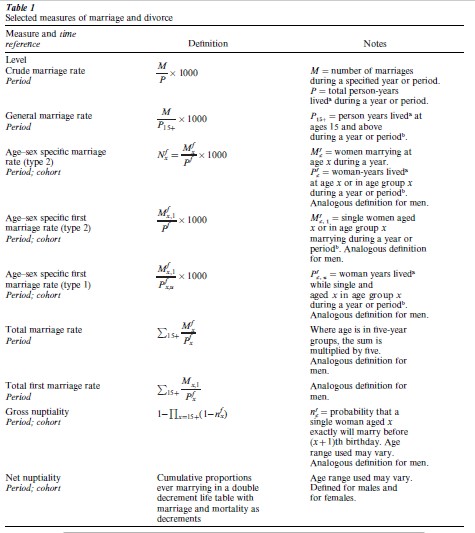
The most basic of the ‘flow’ indicators are the crude marriage rate, defined as the number of marriages per 1,000 population, and the general marriage rate, defined as the number of marriages per 1,000 population aged 15 (say) and above (those eligible to marry; the legally allowable minimum age at marriage varies between countries). These rates are influenced both by the structure of a population across age and sex (since marriage rates vary by both age and sex), and by the proportions already married. To deal with the second of these, a general marriage rate may be defined per 1,000 unmarried persons. Age–sex variation in rates is handled in the conventional way by defining marriage rates specific by age and sex. Age–sex specific marriage rates may be refined by restricting the denominator to the unmarried. Further detail may also be introduced by calculating marriage rates specific by order of marriage. Such rates can be either of type 1 or 2, as outlined in Demographic Measurement: General Issues and Measures of Fertility. (This terminology is not in widespread use in English.) Thus, the numerator of age–sex specific first marriage rates is confined to first marriages and the denominator may include either single (i.e., never-married) persons (type 1) or all persons (type 2) in that age–sex group. Remarriage rates are generally of type 1, i.e., they express the number of remarriages (by age and sex) per 1,000 divorced and widowed persons, but they too can be calculated in type 2 form (remarriages per 1,000 persons in an age–sex group, irrespective of marital status). All rates may be calculated on either a period or a cohort basis. The crude and general marriage rates can be standardized for age, using conventional standardization methods.

As an adjunct to, or sometimes in place of, period or cohort marriage rates, the cross-sectional distribution of marital status by age and sex may be used to depict the nuptiality of a population. Such figures have the advantage that they can be obtained from any census or survey in which individuals’ current marital status is recorded and so do not require vital registration information or annual population estimates by age and sex. They reflect the past marriage, divorce, and widow(er)hood rates of the various age groups and so do not represent current propensities in the population concerned. However, if detailed marriage histories are collected in a survey, or even only the date of first marriage, marriage rates in preceding years may be reconstructed for what will usually be relatively short time series. Retrospective reports may, of course, be inaccurate.

Measuring the frequency of nonmarital cohabitation and of other types of informal partnerships, such as visiting unions, is less straightforward and hitherto there are no widely-agreed standardized methods of doing so (see Murphy 2000 for a discussion of some methodological issues). Because such partner-ships are, by their very nature, not recorded in vital registration systems, current status information and retrospective questions in cross-sectional censuses and surveys are a primary source of information. In developed nations particularly, where the prevalence of cohabitation has increased substantially in the last three decades or so, and in areas such as the Caribbean, where visiting unions have long been common, the absence of good quality information on informal unions limits the accurate description of the de facto union status of a population. Among the indicators commonly used to evaluate the frequency of informal unions are: the proportion (of all or of the unmarried) currently cohabiting, the proportion of those married (or married at some time) who cohabited with their marriage partner (or with any partner) prior to marriage, and the proportion of informal unions among all unions, formal and informal—all of these being more useful if classified by age and sex. Where suitable data are available, the proportion ever having lived in an informal union by specified ages may be calculated. Analogous measures may be specified for visiting unions.

The crude divorce rate is analogous to other crude rates, being defined as the number of divorces per 1,000 persons in a population. It is influenced not only by the age–sex structure of a population but also by the proportions married by age and sex, and also by the distribution of marriages by duration, since divorce rates are closely tied to duration of marriage. Where data are available, a slightly more detailed measure is to be preferred: divorces per 1,000 existing marriages in a population. (Note that this is not the same as the number of divorces occurring in a year per 1,000 marriages occurring in a year, a measure that is neither recommended nor used by demographers.) As with other events, divorce rates are more informative if specific by age and sex (divorces in an age–sex group per 1,000 married persons in that age–sex group). However, in specifying divorce rates, duration of marriage is usually preferred to age since divorce risk varies substantially by marriage duration. Divorce rates may, if data allow, be specific by both age at marriage and duration of marriage, as well as by sex, since the risk of divorce is generally higher among those who marry at younger ages.

Where birth cohort information is available, the cumulative proportions ever having married by specified ages are useful indicators of both the level and the pattern of marriage within and across generations. Birth cohort proportions ever having divorced or ever having remarried can be obtained for the same purpose, though in this case the figures may be influenced by the cohort proportions ever having married or ever having divorced, respectively. To deal with this issue, it may be more appropriate in some circumstances to calculate the proportions ever having divorced (by duration of marriage) for marriage cohorts, rather than birth cohorts, and to obtain the proportions ever having remarried for divorce cohorts.

1.1.1 Synthetic Or Hypothetical Cohort Measures. The total marriage rate is often used to summarize the overall level of marriage for each sex in a population. It is obtained by adding the (type 2) age–sex specific marriage rates and would, if age–sex specific marriage rates were constant through time, represent the average number of marriages a woman or man would experience in a lifetime. The total first marriage rate is defined similarly as the sum of the age–sex specific (type 2) first marriage rates and can be interpreted as the proportion of women or men who would eventually marry, if age–sex specific first marriage rates were to remain fixed. Both of these summary measures have the same strengths and weaknesses as the conventional (additive) total fertility rate (TFR), to which they are analogous. On the one hand, they are standardized for age and so are an improvement on the crude marriage rate. However, like the conventional TFR they are influenced by timing changes and they do not take account of past history, since they are not standardized for marital status. As a result, a period-specific total first marriage rate can, and has been observed to, exceed one first marriage per person—an impossible result, if it is interpreted as applying to a cohort. measures. Two such summaries of the level of marriage in a population are gross nuptiality and net nuptiality. Gross nuptiality is so called because it assumes that all survive to the latest age considered (usually 50, but sometimes an arbitrarily chosen later age). It is obtained, for each sex, by assembling the age-specific first marriage probabilities (type 1) of the unmarried as a life table and computing the proportions ever marrying (not ‘surviving’) by 50 (or an alternative later age), according to normal life table procedures. Net nuptiality, on the other hand, takes account of the fact that death may intervene before marriage, and thus that marriage and death while single are competing events for single persons. It is obtained by constructing a double-decrement life table, with marriage as one source of decrement and death while single as a second source of decrement. Gross nuptiality may be interpreted as the proportion who would marry if they were to experience at each age the age-specific probabilities of marriage pertaining to a given period and if there were no mortality before age 50 (or by the upper age limit chosen). Net nuptiality, on the other hand, may be taken to represent the proportion of a cohort who would marry by 50 (or some other specified age), if they were to experience, while single and at each age, the probabilities of marriage and of death pertaining to the single in a particular period. A practical difficulty with both gross and net nuptiality is that they require more detailed information than is needed to obtain the total marriage rate—namely first marriages by age and sex together with population estimates by age, sex, and marital status in the case of gross nuptiality, and additionally, mortality rates by sex, age, and marital status in the case of net nuptiality. As with life table proportions ‘surviving’ or ‘not surviving’ in general, they are standardized for age structure.

The level of divorce in a population may also be summarized through hypothetical cohort indicators. Analogous to the total marriage rate is the male or female total divorce rate, defined as the sum of age–sex specific type 2 divorce rates and representing the average number of divorces per person if the age–sex specific divorce rates of the period in question were to remain fixed or were to be experienced throughout a person’s lifetime. As before, a multiplicative life table based indicator is to be preferred to the additive measure. The most common indicator used for the purpose is a life table estimate of the proportions who would divorce by a specified duration of marriage, at the rates current at each marriage duration, if these divorce rates were to be experienced by a couple throughout their marriage. As with analogous multiplicative indicators, this standardizes for the distribution by marriage duration and also takes some account of past history. This is probably the best available summary measure of the divorce propensity implied by current divorce rates, but it is demanding of data and is as subject to biases resulting from timing changes as are analogous measures of fertility and marriage. If successive marriage cohorts are moving to an earlier pattern of divorce, the high divorce rates of early-divorcing couples may be combined with the high divorce rates of later-divorcing couples who had lower divorce rates at early durations, to produce an overall hypothetical proportion ever divorcing that is higher than that of any real cohort. At present, there is no specific name in use for this summary indicator.

1.2 Timing

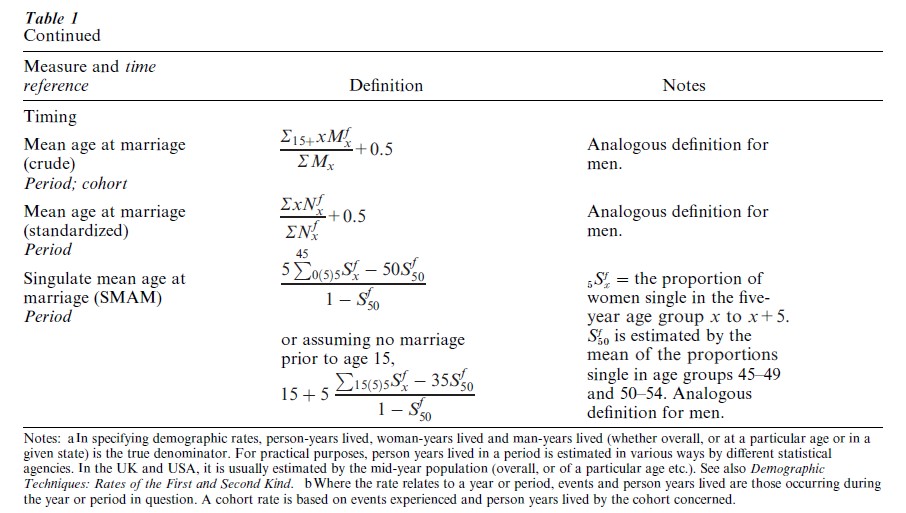
Age at marriage may be calculated from period data in either crude or standardized form, though sources do not always indicate which measure is presented and, as with births, the terms ‘crude’ and ‘standardized’ are not in universal use in this context. The crude mean age at marriage is simply the mean age of those marrying in a period. The standardized mean age at marriage is analogous to the standardized mean age at birth and is the mean of the schedule of age-specific marriage rates (type 2). A crude and standardized median age at marriage may also be obtained. It is often useful to distinguish marriage age by the order of the marriage since the proportion of remarriages among all marriages can vary substantially through time or cross-nationally. Thus, we have the mean or median age at first marriage or at remarriage, either crude (of all those marrying for the first time or for the second or later time) or standardized (using age-specific first or remarriage rates of type 2). Equivalent averages can be calculated for birth cohorts and, as usual, do not require standardization. Mean and median ages at marriage can also be obtained from either gross or net nuptiality tables. Care is needed since the ex-column of a nuptiality table does not give the expected age at or years to marriage. Rather the column gives the expected number of years lived while single at and after age x. Since some never marry, this is not the same as the expected number of years to marriage among those who marry.

Average age at marriage can be estimated from cross-sectional proportions single (never married) by age, by an indirect procedure developed by Hajnal (1953). It gives what is termed the singulate mean age at marriage (SMAM). Based on the hypothetical cohort principle, the procedure is appropriate where marriage rates by age have been reasonably stable and assumes that neither migration nor mortality rates are associated with marital status. Should the proportions single be found to increase over any part of the age range, this indicates that one or more of the assumptions does not hold and so the calculation is not valid. Details are given in Table 1.

Mean and median ages at divorce may be calculated. Of particular interest in relation to divorce is the mean median etc. duration of marriage at which the divorce occurs. A distinction should be made between the duration of marriages in general (those terminated by either divorce or death) and the duration of those marriages that end in divorce. Crude or standardized versions of these indicators may be obtained; for most purposes, standardized indicators are to be preferred.

2. Mortality

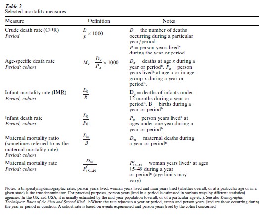
The crude death rate (CDR)—deaths per 1,000 population—is widely used as a basic measure of the level of mortality (see Table 2 for selected mortality measures). It is particularly strongly influenced by the age composition of a population because of the wide variation in death rates by age. Age-specific mortality rates—deaths at a particular age per 1,000 population of that age—are at the next level of detail, usually specific by sex. Where good quality information is available, rates that are specific for single years of age are produced, in preference to five-year age groups. Rates specific by single years of age are of particular importance at the younger and older parts of the age range, since in these age ranges differences in rates between adjacent single years of age may be sizable. Age may be grouped in a variety of ways, according to the refinement required in analysis and the nature of available data. However, even where five-year groups are used, the age groups zero to one and one to four are often distinguished, because of the relatively high death rate of infants, even in low mortality countries.

The measurement of mortality is simplified to some extent by the fact that death occurs ultimately to all and occurs only once. These twin aspects mean that crude and age-specific death rates are necessarily of type 1: the risk of death is universal and, death occurring only once in a lifetime, nobody currently at risk of death can have experienced the event previously. Death rates are so closely and systematically associated with age, and to a lesser extent sex, that specificity by age and sex is adequate for most demographic purposes. Other dimensions of personal time are required much less often in specifying death rates. However, mortality rates may also be specific by social class, race ethnicity, income, area of residence (urban rural or subnational region), marital status, and other such socioeconomic characteristics. Analysis by such factors is of interest in examining social and economic variations in health and for actuarial and public health purposes. With such subspecifications, death rates may also be of type 2.

The infant mortality rate (IMR) is reported and published extensively, partly as a demographic indicator but also as an indicator of socioeconomic development. It is defined as the number of deaths of infants (children under the age of one year) per 1,000 births in a given year. It is, thus, not a rate as normally specified since the numerator is not an estimate of the person-years at risk of the event and will be inaccurate for this purpose to the extent that there are year-on-year fluctuations in births. It is, however, a convenient measure since it can be obtained from simple counts of vital events and does not require population estimates by age. It has a correctly specified counterpart in the infant death rate, the number of deaths of infants (under the age of one year) in a year per 1,000 person-years lived under age one. Several mortality rates are distinguished also during the first year of life, both because of the steep decline in death rates over the first 12 months of life and because of the changing role of endogenous (genetic, intrauterine, perinatal) and exogenous (environmental, external) causes of death. Endogenous causes predominate in the earliest post-partum period, with exogenous factors growing in importance thereafter. The perinatal mortality rate is defined as the number of late fetal deaths plus the number of deaths within one week of birth per 1,000 total late fetal deaths plus live births. The neonatal mortality rate is defined as the number of deaths within one month (28 days) of birth per 1,000 live births, and the post-neonatal mortality rate as deaths between 28 days of birth and one year of age per 1,000 live births. The probability of dying between birth and the fifth birthday is widely referred to in the current demo-graphic literature as the child mortality rate, though the latter is more correctly defined as the number of deaths of children under the age of five years per 1,000 person-years in the age group. The probability definition (also sometimes termed child mortality risk) has become widespread because under-five mortality is of particular interest in high-mortality, less-developed societies, for which the indirect methods used to evaluate child mortality estimate a cohort probability rather than a rate. High-mortality societies do not usually have good vital registration statistics and it can be difficult to formulate accurate assumptions about the average number of years lived by those who die, and thus to obtain an estimate of person-years lived.

Table 2 Selected mortality measures

Maternal deaths are those that occur during pregnancy or within 42 days of the end of the pregnancy, due to a cause related to the pregnancy or a condition aggravated by pregnancy; the term thus includes abortion-related deaths. Maternal mortality is most often represented by the maternal mortality ratio: the number of maternal deaths per 100,000 live births in a period. This indicator is referred to by many authors and in many sources as the maternal mortality rate, although it is not in fact a true rate. Strictly, the maternal mortality rate is the number of maternal deaths per 100,000 women of reproductive age in a period, and some authors employ the term in this sense. It should be clear from the context which definition is in use.

Mortality specific by cause of death, of which maternal mortality is an instance, is the principal way in which mortality indicators are disaggregated be-yond age and sex. The International Classification of Disease, currently produced and revised from time to time by the World Health Organization, is the standard scheme by which cause of death is classified. Measures of mortality by cause of death are of two kinds. Cause-specific mortality rates refer to the number of deaths from a particular cause during a period per 100,000 population, and may be specific also by age and/or sex. A multiplier larger than 1,000 is normally used for the purpose, since deaths from any one cause will usually be relatively small in number. Cause-specific mortality ratios, on the other hand, relate to the percentage of all deaths that result from a particular cause, either overall or by age and sex, and are of value where information on population denominators is inaccurate or unavailable. Proportional mortality analysis is used particularly in the study of occupational mortality.

2.1 Age Standardization

Because of the substantial variation in death rates by age (and in age structure across time and place), cross-national, areal, or time comparisons of the level of mortality require that death rates are standardized for age. Direct standardization, in which a standard age distribution is employed, yields a directly standardized death rate. Indirect standardization, in which a standard set of age-specific mortality rates is chosen, yields two indicators: the standardized mortality ratio (SMR) and the indirectly standardized death rate. The SMR gives an index figure expressing the level of mortality in the index population relative to that of the standard population, set usually to 100: it is simply the ratio of observed to expected deaths in the index population, with expected deaths based on the standard population’s age-specific rates. Multiplying the SMR by the CDR in the standard population gives the indirectly standardized death rate in the index population. Direct standardization requires that the age-specific mortality rates are known and precisely estimated in the populations to be standardized. Where the age-specific rates are either unknown or subject to sizable errors, the indirect method must be used. Statistical theory singles out a version of indirect standardization as optimal when a multiplicative model holds for the force of mortality.

2.2 Life Expectancy And Life Tables

Life expectancy at birth, e , can be considered both an indicator of the ‘timing’ of mortality and also a summary of the overall level of mortality in a population. It measures timing in that it represents the expected or average number of years lived by a person or group subject, throughout their lifetime, to a given set of age-specific mortality rates. Because death occurs universally and removes an individual permanently from the population, any increase in death rates at any age is necessarily reflected in a shorter life expectancy, while a decline in death rates at any age is necessarily accompanied by an increase in life expectancy. The expectation of life is influenced both by the level of mortality in a population and by the pattern of mortality by age. As a result, two populations with the same overall life expectancy may differ in their patterns of age-specific death rates. Life expectancy is calculated from a life table, and so is standardized for age. The life table in question may be based on the age-specific mortality rates obtained in a calendar period or those of a birth cohort. Where based on a period life table, the expectation of life and other life table functions are synthetic cohort measures and share the shortcomings of all synthetic multiplicative measures.

The life table is a central analytical technique in demography, having a large variety of uses. It is, however, fairly demanding of data since it requires information on age-specific death rates and thus on the distribution of deaths by age as well as population estimates by age. Because detailed data of this kind are often unavailable for historical populations and for less developed nations, sets of model life tables have been developed corresponding to varying levels and patterns of mortality (Coale et al. 1983, United Nations 1982). Such compilations allow estimates of the level and/or age pattern of mortality to be made from information that is insufficient in itself to determine these.

3. Migration

Along with births and deaths, migration is the final component of population change. Migration is classified according to whether it is into an area (in-migration) or out of an area (out-migration). The sum of in-and out-migration is termed gross migration and the difference between them, in-migration minus out-migration, is known as net migration. For many purposes it is the absolute values of these quantities that are of interest. Crude and specific rates are also used. The crude in-migration (or immigration) rate is the number of in-migrants per 1,000 population and the crude out-migration (or emigration) rate the number of out-migrants per 1,000 population. The crude gross migration rate is the sum of these and the crude net migration rate is the difference between them. Like other demographic events, migration is patterned by age and so rates of all four kinds may be specific by age. For example, the age-specific out-migration rate is the number of out-migrants of a given age per 1,000 population of that age during a specified period. Cumulative migration experience is represented by whether a person has ever migrated from their place of birth (lifetime migration) or during a specified time (e.g., the last year, the last five years). Migration can be decomposed further according to types of area be-tween which the move was made: for example, between or within urban and rural areas.

4. Population Growth

The difference between the crude birth rate and the crude death rate is known as the crude rate of natural increase (CRNI) and represents the rate at which a population is growing or declining in a year purely as a result of vital events. Since migration also influences population growth, the overall population growth rate is CBR–CDR± the crude net migration rate. Where population growth rate is inferred from the change in total population during a period of t years, the growth rate is estimated as r =ln (P_t /P₀)/ t. The intrinsic rate of natural increase is a theoretical quantity, referring to the growth rate of a stable population having a fixed set of age-specific mortality and fertility rates. It can be calculated for a real population, but should be interpreted with care since it represents the growth rate that would be obtained in the hypothetical circumstance that current age-specific rates were to remain fixed and that the population were closed to migration. The difference between the actual population growth rate and the intrinsic rate of natural increase is between the observed growth rate and the hypothetical growth rate that would apply if current vital rates were to obtain in a stable population. While the GRR and NRR may be calculated for actual (empirical) populations, an important proviso must be borne in mind: since the NRR accurately reflects growth prospects only in populations that are stable, when calculated for an actual population it takes no account of prospective growth decline resulting either from migration or from future changes in mortality, nor does it take account of the growth potential inherent in population age structure. The same is true of the total fertility rate (TFR). A TFR of 2.1 in low-mortality countries is widely referred to in the demo-graphic literature as ‘replacement level fertility,’ that is, the level of fertility necessary for population replacement in the long run. But this is potentially misleading. Low-mortality populations with a TFR of below 2.1 can and do continue to grow because of in-migration, declines in mortality, and/or population momentum. Equally, low-mortality populations with a TFR of 2.1 or more can and do decline because of out-migration, changes in mortality, and/or population momentum.

Bibliography:

1. Alderson M R 1982 Mortality, Morbidity and Health Statistics. Macmillan, Basingstoke, UK
2. Coale A J, Demeny P, Vaughn B 1983 Regional Model Life Tables and Stable Populations, 2nd edn. Academic Press, New York
3. Hajnal J 1953 Age at marriage and proportions marrying. Population Studies 7: 111–36
4. Murphy M 2000 The evolution of cohabitation in Britain, 1960–95. Population Studies 54: 43–56
5. Preston S, Heuveline P, Guillot M 2000 Demography. Measuring and Modelling Population Processes. Oxford University Press, Oxford, UK
6. Shryock H S, Siegel J S 1976 The Methods and Materials of Demography, condensed edn. Academic Press, New York United
7. Nations 1982 Model Life Tables for De eloping Countries. Population Studies Series No. 77, United Nations, New York