Formal Demography Of Families And Households Research Paper

1. Classification By Subject Matter

Three types of relationships between individuals can be distinguished (Ryder 1987):

(a) Consanguineal relationships run via the fundamental parent–child relation. Any two persons sharing a common ancestor, i.e., linked by a sequence of birth events, are said to be related by blood.

(b) Co-residence relationships are between persons living together. A foolproof definition of co-residence does not exist (think, for instance, of student housing, lodgers, or part-time households), but ‘sharing roof and manger’ is not bad for a start.

(c) Conjugal relationships are between individuals who are married to each other. In fact, living together in marriage is a special form of co-residence. To many people, the bond of marriage is so special that it is (almost or fully) put on the same footing as the consanguineal bonds mentioned under (a). In modern societies, the traditional marriage is gradually replaced by cohabitation (consensual unions). In these societies, ‘being married’ is more and more replaced by the more neutral ‘living together as a couple,’ which includes both formal marriages and consensual unions, and frequently also includes homosexual cohabitation. The United Nations. Statistical Division (1998) explicitly recommends: ‘Couples living in consensual unions should be regarded as married couples’ (p. 67).

The broad field of family and household demography studies all these links between individuals, in their own right but also in relation to other demographic processes (e.g., migration of household, mortality patterns in kin groups). Within the broad field, several subfields can be identified, according to the type of relationship on which they concentrate: (a) Demography of kinship studies links of type (a) and (c).

(b) Demography of households studies links of type

(b), but also of type (c) since ‘living together as a couple’ is a special form of ‘living together.’

(c) Demography of the family studies the simultaneous links of type (a) and (c), on the one hand, and of type (b), on the other: a family is a group of co-resident kin.

(d) Demography of marriage studies links of type (c).

2. Data Issues

The data sources for household and family demography are the same as for demography in general: censuses, population registers, surveys (in kinship studies, genealogies are also sometimes used). However, definitional problems are particularly strong in household and family data.

There are two sets of definitional problems. The first relates to criteria for establishing whether or not a certain relationship exists between two persons. Examples of such problems include:

(a) Two persons (e.g., a mother and a student child) live together during weekends only. Do they belong to the same household?

(b) Two persons form a household. How to judge whether they ‘live together as a couple’?

(c) Two students live in an apartment, occupying separate rooms but sharing kitchen and bathroom. Do they count as one or as two households?

The second group of definitional problems relates to criteria for classifying households and/or family into categories, like those used in published household statistics. Examples include:

(a) A woman lives with her 30-year old son. Should this household be termed a lone-parent household?

(b) A lone mother cohabits with a new partner. Is this a ‘couple with children’ household, or rather a ‘one-parent family plus other(s)’?

Such definitional degrees of freedom result in actual definitional differences, the consequences of which are potentially very large (Keilman 1995). Therefore, demographers must be well aware of the precise definitions underlying their household and family data. In descriptive studies, definitional differences can seriously distort international or intertemporal comparisons. In modeling exercises, it is crucial that model parameters are derived from data that are definitionally consistent with the variables in the model. In order to stimulate international comparability of household and family data, the United Nations has specified detailed, extremely useful recommendations for data collection, definition, and tabulation in population and household censuses (United Nations, Statistics Division 1998).

3. Unit Of Analysis

A major problem in the formal demography of families and households is whether the group or the individual should be taken as the primary unit of analysis. Almost by definition, the behavior of the individuals within the group are highly interdependent. Therefore, analyzing the behavior of the group cannot be done without proper account of the characteristics of its members; conversely, analyzing the behavior of the individual cannot be done without proper account of the characteristics of the group (including those of the other individuals in the group).

Today, most family and household demographers agree that it is most convenient to work at the level of Individuals. The main reason for this is that, unlike individuals, groups do not have a clearly defined origin and destination in time since members can enter and leave all the time. Thus, modern practice is to define a group in terms of its members and the relationships between them, rather than defining individuals in terms of the group to which they belong.

Because of strong interdependence of within-group behavior, proper modeling of individual family or household members’ behavior requires sufficient information on the characteristics of the other individuals involved. In microlevel data, this implies the inclusion of pointers or reference variables to other individuals in the dataset, with sufficient detail on the type of the relationship to that other individual. A main advantage of such data is that it can provide very rich descriptive information on different family and household types, as opposed to standard census breakdowns by just a few main categories.

Naturally, when using sample survey data, proper account should be given to the representativeness of the data at different units of analysis. For example, a random sample of individuals is not representative at the household level, since large households will be over-represented. Weighting schemes must be used to correct this and other potential distortions.

4. Models In Family And Household Demography

A model is a simplified, quantitative description of reality. In family and household demography, models provide a formal description of the quantitative relationships between family or household characteristics and their demographic determinants and consequences (Bongaarts 1983).

At the heart of any modeling exercise lies the specification of the state space: the representation of the components of the system of interest. At the level of the Individual, the state space consists of a number of characteristics or attributes (e.g., age, sex, position in the household, age of spouse, number of children), each of which can take a certain value. At the population level, the state space consists of all possible combinations of attribute values: it is a breakdown of all individuals comprising the population by relevant characteristics.

The ultimate purpose of model building is to obtain an understanding about this multidimensional breakdown of the total population. A classical demographer is satisfied with a breakdown by age and sex. A marriage demographer would want to add at least ‘marital status’ as an additional variable. A kinship demographer would want to add a complete breakdown by number of living children, grandchildren, siblings, parents, and so on. A household demographer would want to have, next to age and sex, variables like household size and household type, in a classification that is sufficiently detailed for the research or policy problem at hand. All these demographers have in common that they want to understand why an observed population breakdown is how it is; how particular changes in behavior (for example, total fertility level) would change this breakdown; or how the currently observed breakdown will develop over time (forecasting).

The particular problem in household and family models is that the relevant state space is potentially very large and complicated. This has forced family and household demographers to sacrifice all kinds of descriptive, behavioral, and/or conceptual detail. Evidently, the result is that existing household and family models reflect a wide range of different modeling strategies. Three important classes of these strategies are discussed in the sections below.

4.1 Severing The Link

As said before, family and household demography is all about relationships between individuals. A particularly important type of ‘sacrifice’ frequently made by family and household demographers is to discard most of the information on the characteristics of the individuals with whom a particular relationship exists. For example, in the case of a marriage model, a woman aged 40 and married to a man aged 42 is classified as being a married woman aged 40: the information about the age of the husband is discarded. Without discarding, the total population would require a table of 2×100×(1+100)=20,200 cells (2 sexes, 100 age groups, 1 for nonmarried, 100 for married by age of spouse); with discarding, a table of 2×2×100=400 cells is sufficient (2 sexes, 2 for nonmarried vs. married, 100 age groups). In other words, a frequently used modeling strategy is to collapse all information on all individuals to whom person x has relevant relationships into just a few attributes of person x, thus in fact ‘severing’ the explicit link to those related individuals.

An example of this ‘severing the link’ strategy is provided by marital-status models of the multistate type. Here, individuals are classified by sex s (m for men, f for women), age x, and marital status i, where i can take the following values: N for never married, M for married, D for divorced, W for widowed. The development over time of the population is described in terms of e ents, which are changes in the attributes of the individual members of the population. For example, next year’s 31-year old married female population is given by (ignoring migration):

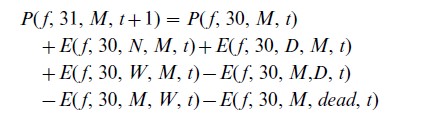
where P(s, x, i, t) denotes the population at the start of year t of sex s, age x, in marital status i, and E(s, x, i, j, t) denotes the number of individuals of sex s and age x who during year t experience an event from position i to position j. The various numbers of events depend on the size of the relevant population at risk of experiencing the event, and on the rate at which individuals in the population at risk experience the event. For example, the number of women who marry for the first time at age 30 in year t, i.e., E( f, 30, N, M, t), equals the product of two factors: the number of never-married 30-year old women P( f, 30, N, t), and the first-marriage rate for 30-year old women M( f, 30, N, M, t).

Given a full set of age-, sex-, origin-, and destination-specific rates, the population by age, sex, and marital status can be projected forward in age and time. Also, a marital-status life table can be calculated. However, a crucial characteristic of this model is that marital-status events for one sex are essentially in- dependent of the demographic situation for the other sex. As a result, in this model it is not guaranteed that the resulting population flows for men and women will be mutually consistent. For example, the number of married men having a divorce should equal the number of married women having a divorce, but there is no mechanism in the model to ensure this equality. This problem is known as the two-sex problem in nuptiality models (Keilman 1985a). It is a direct consequence of the fact that the explicit link between marriage partners is missing. There are several solutions to the two-sex problem, each of which introduces fresh problems:

(a) To restore the link between marriage partners. This greatly expands the state space, since married persons must be simultaneously classified by own age and by the age of their spouse. It also greatly complicates the modeling of numbers of events, since rates must be defined for all combinations of male and female ages and marital statuses.

(b) A slightly different way of restoring the link between marriage partners is to recast the model in terms of microsimulation. See Sect. 4.2.

(c) To concentrate on one sex (usually: women) only. This is convenient, but obviously unrealistic.

(d) To introduce an adjustment mechanism, by which aggregate numbers of events (i.e., aggregated over all ages) are forced to satisfy certain requirements. For example, if the model initially produces 1,000 male divorces and 800 female divorces, male divorces are adjusted downward and female divorces upward to result in, say, 900 divorces for each sex. Such procedures are called consistency algorithms (Keilman 1985b, Van Imhoff 1992). Although such algorithms can be given a satisfactory behavioral interpretation, they nevertheless have an artificial ring and are certainly rough approximations only.

(e) A combination of the previous two ‘solutions’ leads to consistency algorithms that are one-sex dominant. For example, in a female-dominant marital status model, the total number of male divorces is determined by the female married population and female divorce rates.

Marital status models are by no means the only models in which ‘severing the link’ leads to consistency problems. All household and family models which are of the multistate type suffer from essentially the same problem.

4.2 Macro vs. Micromodels

In principle, an algebraic representation of a model can be manipulated to study the model’s properties. If the model is not too complicated, it could be analyzed in this way. Because family and household models easily get quite complex, analytic models are rare in family and household demography. A good example of an analytic model (although valid under a number of quite restrictive assumptions only) is the kinship model of Pullum (1982).

For more complex models, analytic manipulation becomes infeasible, so that numerical simulation methods have to be used to study the implications of the model. Here, two fundamentally different strategies can be distinguished: macrosimulation vs. microsimulation (Van Imhoff and Post 1998).

In macromodels, numbers of events (e.g., ‘first marriages to women aged 25’) are obtained by applying rates (e.g., ‘first-marriage rate for 25-year old women’) to a group of individuals of a certain size (e.g., ‘number of never-married women aged 25’). In micromodels, events are obtained by applying probabilistic decision rules (Monte Carlo experiments) to Individual persons, separately for a number of individual persons. To follow the example of first marriages: for each individual never-married woman aged 25 in the database, draw a random number between 0 and 1; if this random number is less than the first-marriage probability, the woman is deemed to marry, otherwise she remains unmarried.

In macrosimulation, the calculations are carried out in terms of the cells in the aggregate cross-classification table: for each cell, the model should evaluate how the number it contains will change over time. Microsimulation, on the other hand, does its calculations in terms of the individual records: for each individual, the attribute vector is updated according to the specifications of the model and the results of the Monte Carlo experiments. The storage and retention of information in microsimulation occurs via a list of individuals and their attributes; in macrosimulation this is done via the aggregate cross-classification table. If there are K attributes and M_i categories for attribute i=1… K, the table at the macrolevel consists of M₁×M₂× …×MK cells; in contrast, at the microlevel a total population of N individuals can be described by a matrix with N×K cells. For most applications where a relatively large number of attributes is considered, the size of the aggregate table is much larger than the size of the list. This is particularly the case in household and family models, where characteristics of the individuals to whom relationships exist need to be included. In macromodels this would lead to incredibly large tables.

In micromodels, contrary to macromodels, it is quite easy to keep links between individuals intact, simply by including in the individual records of the database some reference numbers (pointers) to other records (persons) in the database. As a result, the consequences of an event that is simulated for one person can be easily determined and updated for the other persons involved. Thus, the two-sex problem or more generally the consistency problem discussed in the previous section is more or less ‘automatically’ solved in micromodels. The other side of the coin is that, for events that involve creating a new link between individuals, a matching problem has to be solved (e.g., if a woman is simulated to marry, a concrete husband must be identified).

Another main advantage of microsimulation is that it can provide very rich output. The output of a microsimulation model consists of a database with individual data that can be aggregated in an almost infinite number of ways. Compare this with the situation in macromodels, where the aggregation scheme is fixed once the model (i.e., the state space) has been specified. Apart from detailed cross-sectional counts, the microsimulation database can also be used to construct longitudinal information, e.g., in the form of individual biographies.

In short, microsimulation offers three main advantages that are of particular relevance in family and household demography: it can handle a large state space; relationships between individuals can easily and explicitly be retained; and it provides richer output.

This does not automatically imply that microsimulation is the ideal methodology for family and household modeling. As always, these advantages are bought at a cost, and the cost can be heavy. The most important drawbacks of microsimulation are twofold: first, the model results are subject to random variation, and the degree of this randomness gets larger as more explanatory variables are included; second, it takes a lot of time and effort to construct a concrete microsimulation application.

4.3 Dynamic vs. Static Models

Populations change over time, and so do household and family structures. Thus, if a model is to describe this change, is must always contain the time element in one way or another. In this sense, all demographic models are dynamic by definition. However, there are many ways in which time can be included into a model. Merely adding an index t to all model variables and parameters hardly warrants the term ‘dynamic.’ A truly dynamic model should not only specify what the system looks like 10 years from now, but also how the system is supposed to get from here to there. In other words, the processes that underlie the changes in the system variables should be explicitly included in the model. In a truly dynamic model, the focus is on the events of formation and dissolution of relationships between individuals. The LIPRO household model belongs to this category (Van Imhoff and Keilman 1991, Van Imhoff 1995).

In contrast, static models do little more than compare household and family structures at different points in time, thus essentially treating the underlying processes of household and family formation and dissolution as a black box. The classical headship ratio models belong to this category. The headship ratio is the proportion of household heads in a population category, e.g., ‘80 percent of all 40-year old males are head of a household.’ If from a population forecast we know that the number of 40-year old males will increase from 1,000 to 1,500, and we extrapolate that the headship ratio for 40-year old males will increase from 80 percent to 90 percent, then it follows that the number of households headed by a 40-year old male will increase from 800 to 1,350. With headship ratios for all ages and both sexes, a full population forecast can in this way be easily converted into a forecast of the number of (private) households. Several generalizations of the classical headship ratio model exist (Kono 1987). However, they all suffer from the disadvantage that the headship ratio is a static concept: the model cannot tell us why the current ratio of 80 percent will increase to 90 percent.

In a way, the dynamic vs. static issue is gradual rather than fundamental. For instance, if a demographic forecaster hypothesizes that marriage rates will fall by 10 percent between now and 10 years into the future, one could argue that the marriage component of the model is static since the demographic forecaster does not specify how the marriage rates are going to fall. Similarly, the headship ratio method is generally termed static since the changes in age-specific headship are not explicitly specified; however, the changes in the age-specific population size to which these headship ratios are applied are explicitly modeled, so the headship ratio model is dynamic at least to some extent.

In fact, leaving some model variables static rather than ‘truly’ dynamic is an effective strategy to reduce the complexity of the model. The decision of where to stop making variables dynamic is governed by the fundamental tradeoff between information intensity on the one hand, and the capacity to make meaningful predictions on the other. This tradeoff must be faced in every effort of modeling human behavior.

The household model used by Statistics Netherlands for its official household forecasts for The Netherlands is a nice example of a carefully constructed mixed dynamic-static household model (De Beer 1995). This model consists of two layers. The first layer is a multistate marital status model, producing forecasts of the population by age, sex, and marital status. In the second layer, each combination of age, sex, and marital status is distributed over various household positions (e.g., living alone, with partner, as lone parent, as dependent child, etc.), using household position proportions which are extrapolated into the future. The rationale for this strategy is that the available statistical data are sufficiently reliable to allow a dynamic approach to nuptiality, but do not warrant a dynamic treatment of household formation and dissolution. The resulting model is dynamic to the extent that household events are related to nuptiality behavior.

Bibliography:

1. Bongaarts J 1983 The formal demography of families and households: An overview. IUSSP Newsletter 17: 27–42
2. De Beer J 1995 National household forecasts for The Netherlands. In: Van Imhoff E, Kuijsten A, Hooimeijer P, Van Wissen L (eds.) Household Demography and Household Modeling. Plenum, New York London
3. Grebenik E, Hohn C, Mackensen R (eds.) 1989 Later Phases of the Family Cycle. Clarendon Press, Oxford, UK
4. Keilman N W 1985a Nuptiality models and the two-sex problem in national population forecasts. European Journal of Population 1: 207–35
5. Keilman N W 1985b Internal and external consistency in multidimensional population projection models. Environment and Planning A 17: 1473–98
6. Keilman N W 1995 Household concepts and household definitions in Western Europe: Different levels but similar trends in household developments. In: Van Imhoff E, Kuijsten A, Hooimeijer P, Van Wissen L (eds.) Household Demography and Household Modeling. Plenum, New York London
7. Keilman N W, Kuijsten A, Vossen A (eds.) 1987 Modelling Household Formation and Dissolution. Clarendon Press, Oxford, UK
8. Kono S 1987 The headship rate method for projecting households. In: Bongaarts J, Burch T K, Wachter K W (eds.) Family Demography. Clarendon Press, Oxford, UK
9. Pullum T W 1982 The eventual frequencies of kin in a stable populations. Demography 19: 549–65
10. Ryder N 1987 Discussion. In: Bongaarts J, Burch T K, Wachter K W (eds.) Family Demography. Clarendon Press, Oxford, UK
11. United Nations. Statistical Division 1998 Principles and Recommendations for Population and Housing Censuses, Revision 1. United Nations, Department of Economic and Social Affairs, Statistics Division, Statistical Papers Series M No. 67 Rev.1, New York
12. Van Imhoff E 1992 A general characterization of consistency algorithms in multidimensional demographic projection models. Population Studies 52: 159–69
13. Van Imhoff E 1995 LIPRO: A multistate household projection model. In: Van Imhoff E, Kuijsten A, Hooimeijer P, Van Wissen L (eds.) Household Demography and Household Modeling. Plenum, New York London
14. Van Imhoff E, Keilman N 1991 LIPRO 2.0: An Application of a Dynamic Demographic Projection Model to Household Structure in The Netherlands. Swets & Zeitlinger, Amsterdam Lisse
15. Van Imhoff E, Post W 1998 Microsimulation methods for population projection. Population 52: 889–932