Cohort Analysis Research Paper

1. Cohorts

Cohorts as analytic entities appear in the social sciences, the life sciences, epidemiology, and else-where. A cohort can be a set of people, automobiles, trees, whales, buildings; the possibilities are endless. System entry can refer to birth—a person is born, or to any dated event—a machine is assembled on a particular date. A set of individuals who begin serving a prison term at the same point in time might also define a cohort for certain purposes, in which case ‘birth’ refers to initiation into a particular role system and ‘age’ becomes duration (time since system entry). The breadth of the time interval that defines membership in a particular cohort depends on analytic considerations and the nature of the phenomenon under study.

The main difficulties inherent to cohort analysis can be illustrated with data from the NORC General Social Survey, a national sample survey conducted annually or biennially in the United States. Respon- dents in this repeated cross-sectional survey are queried about their emotional wellbeing. Each cell in Table 1 shows the percentages, organized by age and survey year, of those who identified themselves as being ‘very happy.’ Each row shows how happiness levels change across survey year (period) for people within a given age group. Each column reveals age variation in any survey year. The diagonals permit tracking of a single birth cohort over time. Those aged 20–29 in 1973 were born between 1943 and 1953, as were those aged 30–39 in 1983, and those aged 40–49 in 1993. Ten-year age categories lead here to cohorts operationalized as individuals born in contiguous 10-year intervals.

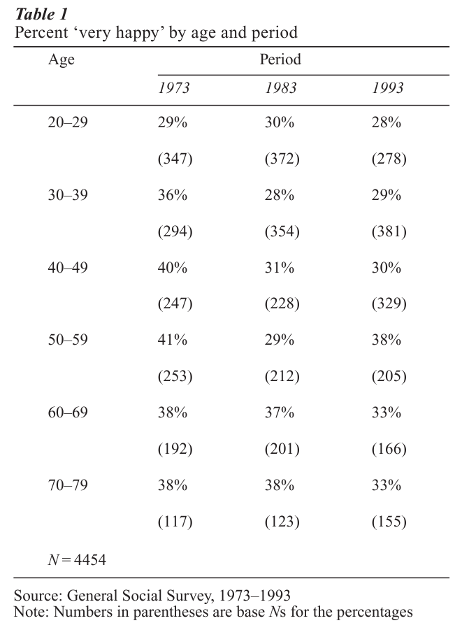
Nominal attempts to extract information from Table 1 would summarize percent ‘very happy’ by rows, columns, and diagonals. The most immediately visible pattern is the association between age and happiness. In all three periods the percentages of respondents who identify themselves as ‘very happy’ are smaller for those under age 40. This reading of the table ignores the possibility that observed variation is due to birth cohort, with younger cohorts less likely to report being happy. Although visual inspection of the diagonals does not suggest a consistent association between decade of birth and eventual happiness, the absence of an observable relationship does not confirm that no such relationship exists. A potential association between birth cohort and adult happiness may have been obscured by the effects of age and period. Finally, there appears to be little systematic variation between years in percent ‘very happy.’ In this instance, however, a potential association between period and current happiness may have been obscured by age and cohort. A further, linked difficulty is that the data structure is imbalanced. Although periods are represented over all ages, and ages are represented over all periods, the observed age spans of cohorts necessarily differ.

This imbalance cannot be extirpated from analyses that take into account age, period, and cohort simultaneously. Comparable points hold for other data structures supporting the analysis of multiple cohorts.

Table 1 shows that data structures that allow for measurements on multiple cohorts necessarily measure age and period. Furthermore, knowledge of placement on any two of age, period, and cohort determines placement on the third. This dependency can be expressed as:

which raises the questions of whether and how all three of age, period, and cohort can be included in cohort models. The linear dependency between age, period, and cohort, also known as the cohort analysis identification problem, is the point of departure for all modern discussions of techniques of cohort analysis. The identification problem is present irrespective of data structure.

2. Data Structures

Three commonly seen data structures engender cohort analysis (for a fuller discussion of data structures, see Fienberg and Mason 1985). Excluded from this discussion, however, would be the single cross section. Reducing Table 1 to a single column indicates the data structure of a single cross section. With this design, differences on an outcome variable by age can be interpreted either as age or cohort differences. The data structure provides no basis for choosing because there is but a single period. Interpretation of age differences on an outcome as being attributable to factors thought to vary with age or duration requires the assumption that there are no cohort or period differences, or that they are known. Parallel assumptions are necessary for interpreting the age differences as attributable to cohort. Thus, the single cross section does not permit cohort analysis.

Some cross-sectional surveys elicit retrospective data on birth, marital, or other kinds of histories. Figure 1(a) structures this design, a single cross section with retrospective data, as an upper-triangular age by period array with cohorts defined by diagonals.

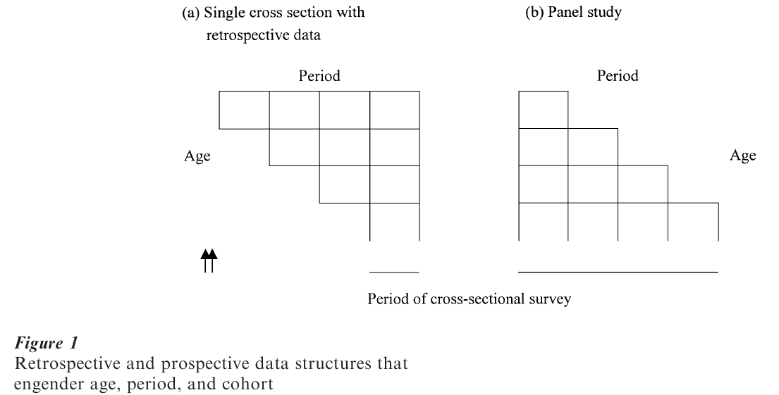
The retrospective data structure provides information on ages, cohorts and periods, and introduces longitudinal information on individuals. When the longitudinal data in this design are used without regard to age, period, and cohort, the analyst is implicitly, and possibly inadvertently, assuming that at least one of age, period, and cohort is not essential. The same point holds for panel study data structures (Fig. 1(b)). A panel study begins with a single cross section, and is followed by one or more panels on the same individuals (units of analysis). This design is intended for the creation of longitudinal data. Figure 1(b) structures the panel study as a lower-triangular age by period array with cohorts on the diagonal. It is triangular because, in the simplest case, panel designs do not replenish the data structure with the addition of new cohorts after the initial cross section. A panel study could also be designed to include new cohorts at successive waves of data collection; the age, period, cohort dependency would remain.

In the replicated cross-section design or time series of cross sections illustrated by Table 1, typically the same individuals are not tracked from one period to the next. However, each cross section can have a retrospective component, and thus this design can be longitudinal. Like the other multiple cohort designs, this structure permits cohort analysis, although the class of models it supports is less rich when retrospective information is unavailable.

3. Cohort Models

Cohort models may be fixed or random effect; terms for age, period, and cohort may enter the model as discrete or continuous; one or more of the age, period, and cohort dimensions may be included in the model via an explicit, substantive measure of that dimension; interactions are possible. These are the most prominent possibilities in the literature on cohort analysis.

3.1 Fixed Effect: Discrete Age, Period, And Cohort

Assume an I J age by period array (Table 1 is a 6×3 illustration), with age groups and period intervals of identical widths. The K = I+J-1 diagonals of the array correspond to cohorts. The basic fixed-effect model treats a parameter (θ_ijk) associated with a response variable as a linear function of discrete age, period, and cohort. Using dummy coding for age, period, and cohort, let:

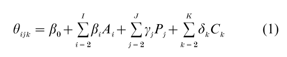
where the A_i, P_j, and C_k (k=i-j+J ) are dummies for ages, periods, and cohorts, respectively. This is a fixed- effect model because inference is conditional on the ages, periods, and cohorts represented by a particular dataset. Although Eqn. (1) manifests usual normalization restrictions (omission of one dummy from each classification), this is insufficient to break the linear dependency between age, period, and cohort. Omission of all terms in one of the age, period, or cohort classifications eliminates the dependency. This is a satisfactory strategy if prior theory and information suggest that age, or period, or cohort is superfluous. On the other hand, if all three dimensions are deemed indispensable to the analysis, the dependency must be eliminated by one or more further restrictions on coefficients if the fixed-effect, discrete model is to be employed. Problems with this approach include col- linearity among terms on the right hand side of Eqn. (1) remaining after additional coefficient restrictions have been introduced, and coefficient bias. Moreover, restrictions that might appear to be innocuously different, such as equating the coefficients of different subsets of adjacent categories, can lead to quite different sets of age, period, and cohort effects, with the various models all fitting the data equally well, or nearly so. One response to the problems of estimating Eqn. (1) is to massively over-identify one or more dimensions. For example, a priori knowledge may suggest that period can be represented by several, rather than many, categories. The data cannot, how-ever, be relied on to contain the information on which to base over-identifying restrictions (Fienberg and Mason 1985, Glenn 1989, Heckman and Robb 1985, Kupper et al. 1983, Mason and Smith 1985, Wilmoth 1990).

3.2 Fixed Effect: Continuous Time

Let age (A), period (P), and cohort (C ) be measured in continuous time, with C P A. Then the continuous time equivalent to Eqn. (1) is:

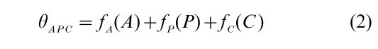
where f_A(A) is an (I-1)th-order polynomial in A, f_P(P) is a (J-1)th-order polynomial in P, and f_C(C ) is a (K-1)th-order polynomial in C. Because of the C=P-A linear dependency, the coefficients of the linear terms for A, P, and C are not estimable. As in the discrete case, at least one linear restriction must still be imposed and in any event the discrete variable approach is generally preferable.

3.3 Random Effect, Discrete Age, Period, Cohort

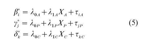
It is possible to view the modeling of age, period, and cohort effects from a Bayesian, hierarchical perspective (Nakamura 1986). In this approach, it is convenient to characterize age, period, and cohort effects through first differences, as in

where A*₁₌A_i-A_i-1, P*_j=P_j-P_j-1, and C*_k= C_k – C_k-1 . The approach assumes that the β*_i,γ*_j, and δ*_k are separately distributed, and that they are random or exchangeable (Nakamura 1986, Sasaki and Suzuki 1987, 1989, Glenn 1989, Miller and Nakamura 1996). The exchangeability assumption requires that within the age dimension, within the period dimension, and within the cohort dimension, all permutations of the first-difference coefficients must be equally acceptable. This assumption makes possible the determination of age, period, and cohort effects without resorting to restrictions on coefficients. To the extent that the assumption fails, and it can when there are shocks (e.g., war, famine, plague, a stock market crash) in the process being modeled, the random effects approach is not a panacea.

3.4 Substantive Measurement Of Age, Period, Or Cohort

When one or more of the age, period, and cohort dimensions, whether represented as discrete or continuous, is replaced by a variable chosen to measure the underlying process thought to be captured by age, or period, or cohort, the linear dependency is almost always broken. Attention is then appropriately focused on the theoretical and substantive merits of the specification. Models that include age, period, and cohort should be thought of as starting points, given their inferiority relative to models that are able to test ideas of how and why a cohort, or period, or age mechanism affects an outcome. Concretely, suppose the cohort dimension is held to reflect the impact of measured variable X, then Eqn. (1) might change to:

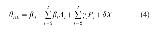
where X is either constant over ages within a cohort, or varies by age within a cohort. Relative cohort size is an example of a variable that could be defined at the birth of each cohort, or allowed to vary as cohorts ‘age’ through the life cycle. Measured variables can also be employed in extensions and revisions of Eqns. (2)–(3). For example, in Eqn. (2) the polynomial in C can be omitted upon inclusion of some function of X (X itself; a polynomial in X; interactions between X and age or period).

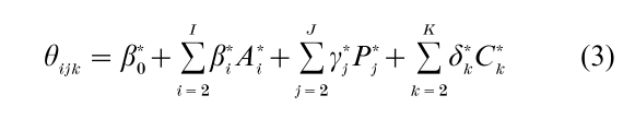
In the extension of the random-effects approach that includes measured variables, cohort analysis becomes a specific case of random effects multilevel analysis. This development can be expected in the course of the continued deployment of Bayesian statistical solutions, because the use of measured variables can enhance the validity of the exchangeability assumption. In the random-effects approach, substantive variables can be written into the model in the following way, for one or all of age, period, and cohort:

where, for example, X_C is a measured variable for cohort, and for simplicity only one measured variable per dimension has been included, and only as a linear term. In this extension it is the τ_iA, τ_jP, and τ_kC that are assumed to be exchangeable within the age, period, and cohort dimensions, and this is likely to be more defensible—because substantively plausible underlying, measured variables should covary with the phenomena that produce shocks. Moreover, the exchangeability assumption becomes comparable to the assumption of a random-error term in a fixed effects approach with measured variables.

4. Interactions

The need for interactions often arises, either for substantive reasons (Converse 1976), or for technical, adjustment purposes (Mason and Smith 1985). It is possible to include interactions in both fixed-and random-effect models, regardless of the presence of measured variables. Fienberg and Mason (1985) elaborate readily implemented strategies for doing so in the fixed-effect framework, using either discrete or continuous age, period, and cohort. Not all inter-actions are estimable, and hence they cannot be added into the model at will.

5. Conclusions

Panel studies, cross-sectional studies with retrospective information, and replicated cross sections (including age by period arrays created from process-generated data) engender the analysis of a response variable as a function of age, period, and cohort as well as other factors. Such analyses must contend with the linear dependency between age, period, and cohort membership. The use of one or more measured variables held to underlie at least one of age, period, or cohort can break the linear dependency. So too can application of credible prior information, whether expressed as constraints on coefficients in fixed-effect models, or as exchangeability assumptions in random-effects or hierarchical models. Measured variables can, of course, be incorporated into both fixed-effect and random-effect models. This strategy is to be preferred, since it makes it possible to test ideas about substantive processes in the most direct way. Models that include age, period, and cohort can also include interactions between these dimensions, though not all such terms have estimable coefficients. Models that do not explicitly consider all three of age, period, and cohort, and yet are based on data structures that permit their inclusion, rest on the implicit assumption that age, or period, or cohort is irrelevant. This assumption should and can be assessed.

6. Further Reading

Fienberg and Mason (1985) discuss the formalization of the identification problem; identifiability of non-linear components; identifiability of certain interactions beyond those implicit in the simultaneous inclusion of age, period, and cohort; polynomial models; and other topics. Kupper et al. (1983) and Kupper et al. (1985) explore in depth several issues raised by the identification problem for the fixed effect discrete case, and take the stance (Kupper et al. 1985) that age-period-cohort models are no more informative than exploratory graphical displays. Ploch and Hastings (1994) illustrate the use of smoothed perspective plots. Robertson and Boyle (1998b) provide an overview of different strategies for graphical display of age-period-cohort data.

In Nakamura’s (1986) Bayesian formulation, identifying linear restrictions are replaced by the assumption of exchangeability of first differences in age, period, and cohort effects (although Nakamura chooses to emphasize the closely related assumption of ‘smooth-ness’). Hodges’ (1998, Sect. 2) development of hierarchical models as linear models contributes to an understanding of how Nakamura’s specification over-comes the singularity of the fixed effects model matrix. Berzuini and Clayton’s (1994) Bayesian formulation, which is focused on second differences of effects, does not solve the identification problem. The social sciences literature in which Nakamura’s specification is used or discussed (Sasaki and Suzuki 1987, 1989, Glenn 1989, Miller and Nakamura 1996) fails to make clear that it is not the Bayesian approach per se that provides an alternative to linear restrictions on coefficients, but rather Nakamura’s particular formulation. Nakamura’s (1986) computational approach has been supplanted by the use of Markov Chain Monte Carlo methods (The BUGS Project 2000).

Robertson and Boyle (1998a), and Robertson et al. (1999) review the largely disciplinary-specific epidemiological literature on the methodology of cohort analysis, which has focused primarily on additive models, and conclude that only the nonlinear components of age, period, and cohort can be used reliably. Holford et al. (1994) employ substantive reasoning about cell malformation in carcinogenesis, develop specifications in which age is inherently nonlinear (e.g., logarithmic) and thus eliminate the identification problem through choice of functional form. Mason and Smith’s (1985) extended study of tuberculosis mortality combines substantive reasoning based on prior information and expectations, uses one body of data to guide modeling of another, includes an interaction term, employs a substantive, measured variable, and concludes that potential interactions require at least as much attention as the identification problem itself.

Hobcraft et al. (1985) focus on theoretical reasons for the use of age, period, and cohort in different areas within demography. Nı Brolchain (1992) takes aim at the relevance of the cohort dimension for under-standing temporal variation in human fertility. Discussions of this kind can help cohort analysts become more substantively grounded. Research using measured variables in place of accounting categories (e.g., cohort size instead of a cohort classification) is not, however, in need of such assistance (Easterlin 1980, Ahlburg and Shapiro 1984, Welch 1979). Blossfeld (1986) provides a persuasive example of the use of massive over-identification within a single dimension.

Bibliography:

1. Ahlburg D A, Shapiro M O 1984 Socioeconomic ramifications of changing cohort size: An analysis of U.S. postwar suicide rates by age and sex. Demography 21: 97–108
2. Becker H A (ed.) 1992 Dynamics of Cohort and Generations Research. Thesis Publishers, Amsterdam
3. Berzuini C, Clayton D 1994 Bayesian analysis of survival on multiple time scales. Statistics in Medicine 13: 823–38
4. Blossfeld H-P 1986 Career opportunities in the Federal Republic of Germany: A dynamic approach to the study of life-course, cohort, and period eff Eur. Sociol. Re . 2: 208–25
5. Converse P E 1976 The Dynamics of Party Support: Cohort Analyzing Party Identification. Sage, Beverly Hills, CA
6. Easterlin R A 1980 Birth and Fortune: The Impact of Numbers on Personal Welfare. Basic Books, New York
7. Elder G H Jr 1999 [1974] Children of the Great Depression: Social Change in Life Experience, 25th Anniversary edn. University of Chicago Press, Chicago
8. Fienberg S E, Mason W M 1985 Specification and implementation of age, period, and cohort models. In: Mason W M, Fienberg S E (eds.) Cohort Analysis in Social Research: Beyond the Identification Problem. Springer-Verlag, New York, pp. 44–88
9. Glenn N D 1989 A caution about mechanical solutions to the identification problem in cohort analysis: Comment on Sasaki and Suzuki. American Journal of Sociology 95: 754–61
10. Heckman J, Robb R 1985 Using longitudinal data to estimate age, period and cohort effects in earnings equations. In: Mason W M, Fienberg S E (eds.) Cohort Analysis in Social Research: Beyond the Identification Problem. Springer Verlag, New York, pp. 137–50
11. Hobcraft J, Mencken J, Preston S 1985 Age, period, and cohort effects in demography: A review. In: Mason W M, Fienberg S E (eds.) Cohort Analysis in Social Research: Beyond the Identification Problem. Springer Verlag, New York, pp. 89– 135
12. Hodges J S 1998 Some algebra and geometry for hierarchical models, applied to diagnostics (with discussion). Journal of the Royal Statistical Society: Series B 60: 497–536
13. Holford T R, Zhang Z, McKay L A 1994 Estimating age, period and cohort effects using the multistage model for cancer. Statistics in Medicine 13: 23–41
14. Kupper L L, Janis J M, Karmous A, Greenberg B G 1985 Statistical age-period-cohort analysis: A review and critique. Journal of Chronic Disease 38: 811–30
15. Kupper L L, Janis J M, Salama I A, Yoshizawa C N, Greenberg E 1983 Age-period-cohort analysis: An illustration of the problems in assessing interaction in one observation per cell data. Commun. Statist.–Theor. Meth. 12: 2779–807
16. Mason W M, Fienberg S E (eds.) 1985 Cohort Analysis in Social Research: Beyond the Identification Problem. Springer Verlag, New York
17. Mason W M, Smith H L 1985 Age-period-cohort analysis and the study of deaths from pulmonary tuberculosis. In: Mason W M, Fienberg S E (eds.) Cohort Analysis in Social Research: Beyond the Identification Problem. Springer Verlag, New York, pp. 151–227
18. Miller A S, Nakamura T 1996 On the stability of church attendance patterns during a time of demographic change: 1965–1988. Journal for the Scientific Study of Religion 35: 275–84
19. Nakamura T 1986 Bayesian cohort models for general cohort table analyses. Ann. Inst. Statist. Math. 38: 353–70
20. Nı Bhrolchain M 1992 Period paramount? A critique of the cohort approach in fertility. Pop. De . Re . 18: 599–629
21. Ploch D R, Hastings D W 1994 Graphic presentations of church attendance using general social survey data. Journal for the Scientific Study of Religion 33: 16–33
22. Robertson C, Boyle P 1998a Age-period-cohort models of chronic disease rates. I: Modeling approach. Statistics in Medicine 17: 1305–23
23. Robertson C, Boyle P 1998b Age-period-cohort models of chronic disease rates. II: Graphical approaches. Statistics in Medicine 17: 1325–39
24. Robertson C, Gandini S, Boyle P 1999 Age-period-cohort models: A comparative study of available methodologies. Journal of Clinical Epidemiology 52: 569–83
25. Ryder N B 1965 The cohort as a concept in the study of social change. Am. Sociol. Re . 30: 843–61
26. Sasaki M, Suzuki T 1987 Changes in religious commitment in the United States, Holland, and Japan. American Journal of Sociology 92: 1055–76
27. Sasaki M, Suzuki T 1989 A caution about the data to be used for cohort analysis: Reply to Glenn. American Journal of Sociology 95: 761–5
28. The BUGS Project 2000 http: www.mrc-bsu.cam.ac.uk bugs Welch F 1979 The effects of cohort size on earnings: The baby boom babies financial bust. Journal of Politics and Economics 87: 565–97
29. Wilmoth J R 1990 Variation in vital rates by age, period, and cohort. Sociological Methodology 20: 295–335