Growth Curve Analysis Research Paper

Growth curve analyses are among the most widely studied and well-developed mathematical and statistical techniques in all scientific research. These analyses have roots in the seventeenth and eighteenth-century calculus of Newton and probability of Pascal, but this research paper is limited to more recent historical developments and other related techniques, such as time-series and dynamical systems analyses are not covered.

1. Growth Cur E Data Collections

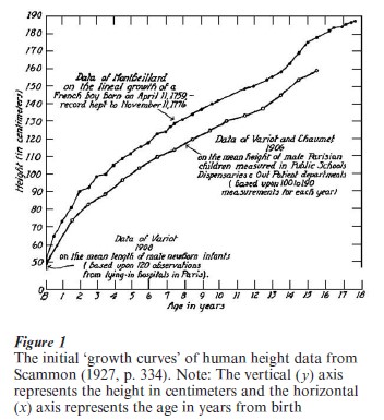
The first reported growth curve data were collected by the French Count de Montbeillard between 1759 and 1777. These data consist of semi-annual measurements on the growth of the height of his son over nearly 18 years. The data were plotted by Scammon (1927) and are presented here in the upper curve of Fig. 1. As Scammon reported

it will be noted that the curve shows the typical four phases which most modern students have observed in the postnatal growth in stature of man, and which are characteristic of the growth of so many parts of the body (p. 331).

The first analysis of these data was by the naturalist Buffon in 1799 and

should be given full credit for the discovery of seasonal differences in growth a full hundred years before the modern investigation of this work (p. 334).

The lower growth curve in Fig. 1 is based on group averages obtained by Variot in 1908 and

it is interesting to note that, while the absolute values of the two series are quite different, the general form of the curve is essentially the same in both instances (p. 335).

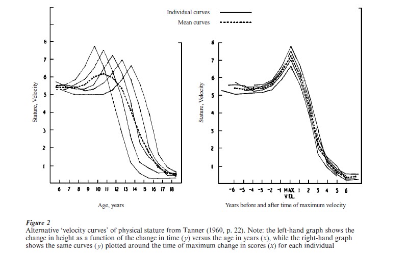
These early growth curves were the precursor to an enormous collection of biological data on growth and change. A more recent illustration comes from the important work of Tanner and his colleagues (see Tanner 1960). In the individual plots of height in Fig. 2: (a) the ‘velocity’ or rate-of-change is plotted at each age and (b) these curves are plotted against their own ‘highest peak velocity.’ This display demonstrated two interesting features of physical growth: (a) persons who start growth at the earliest ages also grow the most but (b) all individuals share a remarkably similar shape in their ‘adolescent growth spurt.’ Extensions of these basic findings on physical growth systems and the contrast of chronological time vs. biological time, are still used in contemporary research.

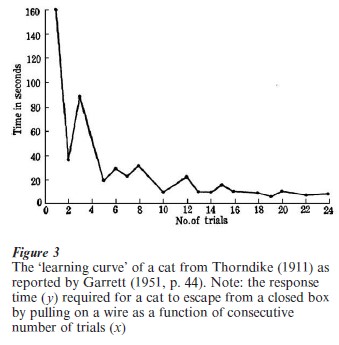
Experimental psychologists have routinely collected different kinds of growth curves. Among the first here were the classical ‘forgetting’ curves collected by Ebbinghaus in the 1880s, whose work introduced the use of quantitative methods in the study of learning and memory and stimulated many experimental data collections. Included here are the ‘curves of improvement’ in studies on telegraphic language by Bryan and Harter in 1897. These principles were also used in the animal learning curve experiments of Thorndike in 1911, and one example of such data appears in Fig. 3. This plot illustrates an example of ‘trial and error’ learning: learning was objectively defined by decreasing response time and the lack of smooth function over trials was considered as error. Thorndike used these growth curves to illustrate several classical principles of learning, including the ‘law of exercise’ and the ‘law of effect’ (see Garrett 1951).

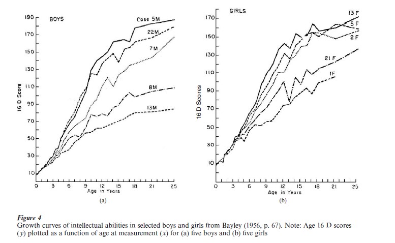
Differential psychologists have also contributed growth data in many different substantive areas. One good example of this tradition is given in the plots of Fig. 4 from work of Bayley (1956). Individual growth curves of mental abilities from birth to age 25 are plotted for a selected set of boys and girls from the well-known Berkeley Growth Study. Because mental ability was not easily measured in exactly the same way at each age, these individual curves were created by adjusting the means and standard deviations of different mental ability tests (i.e., Stanford-Binet, Terman-Merrill) at different ages into a common metric. As Bayley says

they are not in ‘absolute’ units, but they do give a general picture of growth relative to the status of this group at 16 years … These curves, too, are less regular than the height curves, but perhaps no less regular than the weight curves. One gets the impression both of differences in rates of maturing and of differences in inherent capacity (1956, p. 66).

This use of ‘linked’ measurement scales created a novel set of growth data and permitted the use of growth analyses initially derived in other scientific areas.

2. Linear Models For Growth Curve Analyses

The simplest growth models are based on the simplest mathematical functions. The fitting of a straight-line to a set of measurements, a standard procedure in scientific research, was an initial model used by Wishart (1938) in a classic paper on growth analysis. These linear models were quite practical because the calculations used standard statistical assumptions (e.g., independence and normality of the residuals), standard forms of estimation (e.g., Gauss-Markov least squares, maximum likelihood), and standard statistical tests of goodness-of-fit (F-tests, chi-square tests, and likelihood ratio tests).

Another key idea was also introduced by Wishart (1938) when he showed how power polynomials could be used to fit the nonlinear curvatures apparent in growth data. The individual growth curve (consisting of t=1, T occasions) is summarized into a small set of linear orthogonal polynom ial coefficients based on a power-series of time (t, t¹, t²,…t^p) describing the general nonlinear shape of the growth curve. A model of growth data might require a second-order (quadratic), third-order (cubic), or even higher-order polynomial model fitted to the data, but the basic shape of each individual curve could be captured with a small number of parameters.

The organization of individual differences is an important consideration in any contemporary growth model. In the linear model, each individual is assumed to be following a straight line over time, describable by an intercept term and a slope term. The average of these individual scores can be used to describe the overall growth curve for the group, and the individual differences can be considered in the context of other substantive questions, e.g., do the groups under observation differ in intercepts or slopes? In the more complex polynomial models, Wishart suggested a second stage of analysis where these polynomial coefficients describing each individual curve were considered as the underlying scores that co-vary among different individuals. In a quadratic polynomial, for example, a person’s trajectory over time could be summarized using an individual intercept, linear slope, acceleration, and a residual term, and secondary questions could be addressed, e.g., do the groups under observation also differ in acceleration?

This ‘curve-fitting’ or ‘two-stage’ approach was relatively easy to implement using a standard statistical basis for hypothesis testing (e.g., Bock 1975). The simplicity of this approach allowed linear growth models to enjoy widespread use in behavioral studies and become a useful starting point for understanding individual differences in change (e.g., Rogosa and Willett 1985). The persistent critiques of this polynomial approach include some key issues:

(a) the individual parameters can be difficult to estimate, especially for higher-order terms and incomplete data,

(b) even high-order polynomials (i.e., p 4) cannot capture ‘seasonality’ or ‘phase-shifts,’

(c) the substantive meaning of these individual parameters is often in doubt, and

(d) the individual level parameters can be transformed (i.e., rotated) to yield alternative meaning.

These standard critiques are appropriate, and they still apply to many other contemporary forms of growth curve analyses.

More complex linear models have been used to represent growth. A linear model applied to different age segments but with connected critical ‘knot points’ permitted a ‘conjoined’ or linear or polynomial ‘spline’ model (e.g., Bryk and Raudenbush 1992). This kind of spline model is not often used, partly because it is atheoretical, and partly because it may requires a relatively large number of parameters to achieve adequate fit. A more parsimonious organization of individual differences was proposed in the form of ‘latent curves,’ independently defined by both Rao and Tucker in 1958 (cited in Meredith and Tisak 1990). Principal components of the repeated observations were used to reorganize these data into the sum of a small number of unspecified linear functions are fitted to growth data, the shape of the latent curves is determined by the component loadings, and the individual curve parameters are the component scores. The summation of latent curves has roots in classical nineteenth-century work of Fourier as now widely used. In a recent innovation, Meredith and Tisak (1990) showed how these ‘Tuckerized curve’ models could be represented using confirmatory common factor analysis models, used to represent a wide range of alternative models (including most of the models discussed herein), and fitted using structural equation modeling techniques (also see McArdle 1988, McArdle and Bell 2000, McArdle and Woodcock 1997).

3. Nonlinear Models For Growth Curve Analysis

The linear models can be used to describe a variety of nonlinear shapes, but many growth curve models for specific substantive problems have included nonlinear functions of the parameters. For example, Ebbinghaus in 1880 described his forgetting curves using a form of the classic ‘exponential growth’ model. Here the rate of change is a linear function of the percentage of initial size (e.g., compound interest), and individual trajectories rise or fall in nonlinear fashion towards some asymptotic values. In contrast, the nineteenth century Velhurst curve of population growth, an Sshaped ‘logistic curve,’ was used in the early twentieth century by Pearl for many forms of growth. At about the same time Peters advocated an ‘ogival’ curve of growth in ideational learning, Thurstone found that a hyperbolic curve of learning best to fit the norms of many different tests, and both Ettlinger and Valentine demonstrated direct relationships among these functions (see Seber and Wild 1989, Bock and Thissen 1980).

More complex nonlinear models have been used extensively. In about 1825 Gompertz described the growth curve in terms of two exponential accumulations of different rates towards different asymptotes. This flexible model was studied in the first half of the twentieth century by Winsor, used by Medwar to study the growth of chicken hearts, and by Deming for human physical growth, and in studies of learning curves (see Browne and du Toit 1991). Another popular nonlinear model, introduced around 1938 by von Bertalanffy, suggested that an individual’s change in weight was the direct result of the difference in the forces of anabolism and catabolism, with the exact relationship specified by known empirical properties. In subsequent work, Richards challenged the empirical basis of this model, and formally showed how many prior models can be seen as specific solutions of a ‘family’ of deterministic differential equations; specific restrictions led to the exponential, logistic, Gompertz, and von Bertalanffy equations. This work was more recently extended by Nelder and Sandland and MacGhilcrest (1979). (See also Seber and Wild 1989, Zeger and Harlow 1987.)

Attempts to fit a single growth model to observations over a wide range of ages with a minimal set of parameters led researchers to combine aspects of other models. Jenss and Bayley in 1937 proposed a simple composite where a linear part was used to fit the early rapid growth phase and this was added to an exponential part to fit negative acceleration of the later slowing-down phase. A more complex composite model, the sum of multiple logistic curves, was suggested by Robertson in 1908 and Burt in 1937 but only made practical and fully developed by Bock and his colleagues (see Bock and Thissen 1980). In each segment the rate of growth (a) increases early, (b) reaches a maximum (peak growth velocity), (c) decreases towards the asymptote, and (d) the final value of one segment is used as the starting value of the next segment. A novel composite model based on multiple logistic functions was developed by Preece and Baines in 1978 and here the model parameters were supposed to be linearly related to meaningful biological parameters. Simple versions of this new family of curves have proven useful in contemporary work (see Hauspie et al. 1991).

The mathematical elegance of these nonlinear formulations often make it seem that the parameters estimated are related directly to the underlying phenomena and there is a tendency to treat these estimates with direct substantive interpretation. Prior research has show this to be a difficult goal and now it is known that all models permit alternative formulations that may fit equally well. Another important property of growth curves comes when the fixed parameters of the nonlinear curves, the ‘parameters of the means’ also represents the ‘means of the parameters’ of the individual curves. However, classical research by Merrill in 1931, Estes in 1957, Tucker in 1966, and Keats in 1983 has shown this form of ‘dynamic consistency’ does not always hold, even for some of the most popular growth models (e.g., a group exponential). Contemporary statistical models are now constructd carefully to clarify the unique substantive interpretation of nonlinear parameters (see Browne and du Toit 1991, Bock and Thissen 1980).

4. Multivariate Growth Curve Analyses

The collection of multiple variables at each occasion of measurement leads naturally to questions about relationships among growth processes and multivariate growth models. In biological research, early efforts were directed at characterizing the parallel properties of different growth variables. Models were developed originally to deal with the size of two different organs, and early nineteenth-century work was used by Huxley to form a classical ‘allometric’ model where two variables have a constant ratio of growth rates throughout the growth period. Many physical processes were subsequently found to grow in parallel, or in an ordered time-sequence (e.g., Tanner 1960). This work led to more sophisticated models based on systems of differential equations for the size of multiple variables. In one comprehensive multivariate model, Turner in 1978 extended the simple growth principles to more variables and permitted an examination of biologically important interactions based on the size and sign of the estimated parameters (see Griffiths and Sandland 1984).

Multivariate research in the behavioral sciences has relied on advanced versions of the linear growth models formalized by Rao, and Pothoff and Roy (see Bock 1975). The structural models developed within this framework have added measurement models and this includes work on multivariate models of latent curves (McArdle 1988). These structural models have proven useful in testing hypotheses about parallel growth processes across time in multiple psychological variables. In recent examples, McArdle and Woodcock (1997) showed how latent growth of a single common factor of intellectual abilities is a poor representation of multiple abilities data and McArdle (2000) showed how a multivariate dynamic sequence could be fittted using standard structural equations. Current research in this area is focused on an improved understanding of the time-sequences and interactions among multiple behavioral and biological variables.

5. Recent Issues In Growth Curve Analysis

The prior developments in growth curve analysis represent an important but limited class of longitudinal data analyses (e.g., Nesselroade and Baltes 1979, Bock 1975, Pinherio and Bates 2000). These developments have been distinguished by features of the models themselves: (a) the degree of mathematical specification, (b) the way these statistical models are fitted, and (c) the clarity and substantive meaning of the results. In future work, most of these problems are likely to remain under active investigation.

Most contemporary growth curve models can be written in a common symbolic form (Seber and Wild 1989). A general model for a change in the scores over time (often using derivatives dy/dt or differences ∆y/∆t) can be based on some mathematical functional form (f{x}) with unobserved scores (x[t]) and with unknown parameters (β[t]) to be estimated. Additional statistical forms not discussed here can be included, including autoregressive residual error structures, Markov chains, and Poisson processes. The growth functions described here are not an exhaustive listing and future extensions to more generalized functions, and to dynamic and chaotic forms are likely.

Recent research in statistical model fitting is important here too. It is now clear that growth curve models of arbitrary complexity can be fitted to the observed trajectory over time (i.e., the integral) and the unknown parameters can be estimated to minimize some statistical function (e.g., weighted least squares, maximum likelihood), and parameter estimates obtained using nonlinear programming. This generic statistical approach avoids some problems in older techniques, such as fitting a model to a log-scale or directly to the velocity or the analysis of difference score data (Fig. 2). These new techniques make it possible to address the critical problems of forecasting future observations, and further research on Bayesian estimation is the focus of current research here (for details, see Seber and Wild 1989).

This generic model fitting approach also permits a wide range of new possibilities for dealing directly with unbalanced, incomplete or missing data. In early work, linear polynomials were used extensively to deal with these kinds of problems. But recent work on linear and nonlinear mixed and multilevel models have surfaced, making it possible to estimate growth curves and test hypotheses by collecting only small segments of data on each individual (Bryk and Raudenbush 1992, Pinherio and Bates 2000, Verbeke and Molenberghs 2000). These statistical models are being used in many longitudinal studies to deal with self-selection and subject attrition, multivariate changes in dynamic patterns of development, and the tradeoffs between statistical power and costs of person and variable sampling. The statistical power questions of the future are not ‘how many occasions do we need?’ but ‘how few occasions are adequate?’ and ‘which persons should we measure at which occasions?’ (McArdle and Woodcock 1997, McArdle and Bell 2000).

Some of the most difficult problems for future work on growth curves are related to the elusive meaning of the growth model parameters. Growth curve analyses also rely on basic measurement properties including (a) interval scaling, (b) age-and-time equivalence, and (c) substantively meaningful. These issues are key problems in the behavioral sciences and future research is needed to address these fundamental concerns. Multivariate models may be useful here, especially as these models are further extended to a fully dynamic time-dependent form. In any case, empirical information and experimentation will be needed to judge the utility of any growth curve model.

Given the long history of elegant formulations from mathematics and statistics in this area, it is somewhat humbling to note that many of the most insightful growth curve analyses have come from careful visual inspection of the growth curves (e.g., in Figs. 1–4). The insight gained from visual inspection of a set of growth curves is not in dispute now and in fact obvious visual features should be highlighted and emphasized in future research (e.g., Pinherio and Bates 2000). As in the past, the best future growth curve analyses are likely to be the ones we can see most clearly.

Bibliography:

1. Bayley N 1956 Individual patterns of development. Child Development 27(1): 45–74
2. Bock R D 1975 Multivariate Statistical Methods in Behavioral Research. McGraw-Hill, New York
3. Bock R D, Thissen D 1980 Statistical problems of fitting individual growth curves. In: Johnston F E, Roche A F, Susanne C (eds.) Human Physical Growth and Maturation: Methodologies and Factors. Plenum, New York, pp. 265–290
4. Browne M, Du Toit S H C 1991 Models for learning data. In: Collins L, Horn J L (eds.) Best Methods for the Analysis of Change. APA Press, Washington, DC, pp. 47–68
5. Bryk A S, Raudenbush S W 1992 Hierarchical Linear Models: Applications and Data Analysis Methods. Newbury Park, CA
6. Fischer G H, Molenaar I W 1995 Rasch Models: Foundations, Recent Developments, and Applications. Springer, New York
7. Garrett H E 1951 Great Experiments in Psychology. Appleton- Century-Crofts, New York
8. Griffiths D, Sandland R 1984 Fitting generalized allometric models to multivariate growth data. Biometrics 40: 139–150
9. Hauspie R C, Lindgren G W, Tanner J M, Chrzastek-Spruch H 1991 Modeling individual and average growth data from childhood to adulthood. In: Magnusson D, Bergman L R, Rudinger G, Torestad B (eds.) Problems and Methods in Longitudinal Research: Stability and Change. Cambridge University Press, Cambridge, GB
10. McArdle J J 1988 Dynamic but structural equation modeling of repeated measures data. In: Nesselroade J R, Cattell R B (eds.) The Handbook of Multivariate Experimental Psychology, 2. Plenum Press, New York, pp. 561–614
11. McArdle J J 2000 A latent difference score approach to longitudinal dynamic structural analyses. In: Cudeck R, du Toit S, Sorbom D (eds.) Structural Equation Modeling: Present and Future. Scientific Software International, Lincolnwood, IL, pp. 342–380
12. McArdle J J, Bell R Q 2000 Recent trends in modeling longitudinal data by latent growth curve methods. In: Little T D, Schnabel K U, Baumert J (eds.) Modeling Longitudinal and Multiple-group Data: Practical Issues, Applied Approaches, and Scientific Examples. Erlbaum, Mahwah, NJ, pp. 69–107
13. McArdle J J, Woodcock J R 1997 Expanding test-rest designs to include developmental time-lag components. Psychological Methods 2(4): 403–35
14. Meredith W, Tisak J 1990 Latent curve analysis. Psychometrika 55: 107–22
15. Nesselroade J R, Baltes P B (eds.) 1979 Longitudinal Research in the Study of Behavior and Development. Academic Press, New York
16. Pinherio J C, Bates D M 2000 Mixed-effects Models in S and S-PLUS. Springer, New York
17. Rogosa D, Willett J B 1985 Understanding correlates of change by modeling individual differences in growth. Psychometrika 50: 203–228
18. Sandland R L, McGilchrist C A 1979 Stochastic growth curve analysis. Biometrics 35: 255–271
19. Scammon R E 1927 The first seriatim study of human growth. American Journal of Physical Anthropology 10: 329–36
20. Seber G A F, Wild C J 1989 Nonlinear Models. Wiley, New York
21. Tanner J M (ed.) 1960 Human Growth. Pergamon Press, New York
22. Verbeke G, Molenberghs G 2000 Linear Mixed Models for Longitudinal Data. Springer, New York
23. Wishart J 1938 Growth rate determinations in nutrition studies with the bacon pig, and their analyses. Biometrika 30: 16–28
24. Zeger S L, Harlow S D 1987 Mathematical models from laws of growth to tools for biologic analysis: Fifty years of growth. Growth 51: 1–21