Computational Approaches To Model Evaluation Research Paper

1. Modeling As Inductive Inference

The goal of modeling is straightforward: given observed data, identify the underlying system that generated the data. Realistically, modeling is viewed as a learning problem in which we estimate an unknown function from observed data and then use the estimated function to predict the statistics of future data. When modeling, we reconstruct an unknown function based on several sample points in the data space (local subspace) and then apply it globally, throughout the data space. This process of generalizing from a particular instance to all instances is referred to as inductive inference, or predictive inference given the predictive nature of the process and the goals of the modeler. It is at the heart of the scientific enterprise in modern science as well as in engineering.

1.1 Ill-Posedness Of The Modeling Problem

Identifying an unknown function from data samples is an ill-posed problem, meaning that obtaining a unique solution is not in general possible. The reason stems from the reality that there is rarely enough data available (or information in the data) to discriminate between models. Multiple functions may provide equally good descriptions of the data in hand. This problem is known as the curse of dimensionality, which states that for a function defined in high-dimensional space, it becomes increasingly difficult to estimate accurately the function as dimensionality increases, with required sample sizes increasing exponentially with dimensionality (Cherkassky and Mulier 1998). This problem of ill-posedness can be overcome only by introducing external constraints on, and/or prior information about, the data-generating function.

1.2 Model Evaluation: Finding Best Approximation To Truth

An implication of the ill-posedness problem is that the ‘true’ model, the one that generated the data, can never be found in practice. Accordingly, the previously defined goal of finding the true function underlying observations must be modified. A more realistic goal is to find the best possible approximation to the truth, in which the best approximation is defined as the one that generalizes (i.e., infers) best in some defined sense.

2. Bias-variance Dilemma

Formally, a model is defined as a parametric family of probability distributions defined on random variables Y, representing data. An observed sample of size n denoted by a lower case vector y =(y₁, …, y_n) rep- resent realizations (measurements) of Y, which are presumed to be generated from some true distribution g( y) that the scientist seeks to unravel. The scientist, using a family of distributions f( y|θ)’s where θ is a parameter vector on the parameter space Θ, seeks to construct the best approximation to g within the family f.

Let t =E( y) denote the population mean vector of the true distribution g( y), and let z(θ)= (z₁, …, z_n) denote the vector predicted by the model atθ. Also, let the quadratic function

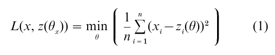
denote a measure of the discrepancy or error between a vector x and the prediction vector z(θ). Note that θ_x denotes the value of the parameter that minimizes the discrepancy measure given a vector x. This function is used to measure the effectiveness or risk of the model family f in approximating the truth g. For example, L( y, z(y)) represents the minimized mean squared error between observed and predicted data, that is, the best possible fit the model provides given data y. Because this quantity changes from sample to sample, a better measure of model effectiveness (or risk) is the expected value of L( y, z(θ_y)), which can be expressed as the sum of two terms:

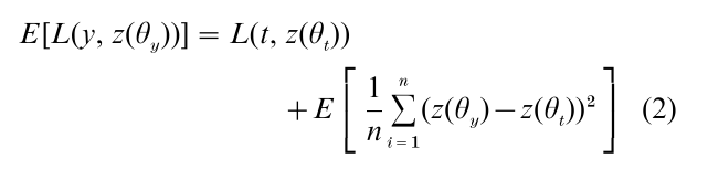
In the above equation E denotes the expectation (i.e., average) taken over all data samples of size n which could be realized under the true distribution g, and t is the mean vector of the true distribution g( y) that has generated the data. Note that the value of the prediction vector z(θ_y) varies across samples whereas z(θ_t) is a fixed constant vector, which can be replaced by E [z(θ_y)].

The left-hand side of the above equation is the expected risk in predicting all data samples given the model family f, and thus it measures the model’s generalizability. The first term of the right-hand side of the equation is the discrepancy between the true mean vector t and the model’s best approximation to t, z(θ_t). Accordingly, this term captures the model’s inability to accurately approximate the truth g, and is called the bias or approximation error. If the model family f includes g as a special case, the bias term becomes zero, and takes on a positive value otherwise. The second term is the expected variability of the prediction vector z(θ_y) around its mean z(θ_t), and is called the variance or estimation error. It captures the lack of information in the sample of finite size about the truth g. As such, this term decreases to zero as sample size n goes to infinity.

To achieve good generalization performance, both the bias and variance of the model family f would have to be minimized at the same time. It turns out, however, that this is not possible because the bias can be minimized by increasing model complexity, whereas increasing complexity will have the detrimental effect of increasing the variance by capturing random error in the data, thereby reducing generalization performance. Complexity refers to the flexibility inherent in a model that enables it to fit diverse patterns of data. In general, a simple model with few parameters has a large bias but a small variance, whereas a complex model (one with more parameters) has the opposite. We thus have a bias-variance dilemma (Geman et al. 1992), with model complexity as the intervening variable that mediates between the two.

The bias-variance dilemma is a useful conceptual framework for understanding the trade-off between approximation error and estimation error, both of which contribute to a model’s generalizability. However, the generalizability measure represented by the sum of bias and variance is not directly observable, because the truth g is unknown, and therefore it must be inferred from observed data.

3. Computational Approaches To Model Evaluation

In order to make the ill-posed problem of modeling into a well-posed one, additional constraints and prior information must be incorporated into the model evaluation process. Computational approaches to the problem differ from one another in how this is accomplished. Structural risk minimization (Vapnik 1992), regularization theory (Tikhonov 1963) and minimum description length (Rissanen 1989) are three major inductive methods of model evaluation.

Briefly, the structural risk minimization method imposes a constraint requiring that, among a set of candidate models, the one that minimizes an expected risk functional should be chosen. Regularization theory chooses among models based on the prior assumption that the unknown function underlying the data is smooth, in the sense that similar inputs map onto similar outputs. The minimum description length method prescribes the constraint that the description length of data should be minimized. Formalizations of these ideas are described in the following sections.

3.1 Structural Risk Minimization

The basic idea of structural risk minimization is to estimate an upper bound of the expected risk, E [L( y, z(θ_y)], in terms of the observable empirical risk, L_emp(y, z(θ_y)), given data sample y and a confidence interval, the value of which depends on a measure of model complexity and sample size, n. For binary classification problems for which y_i =0 or 1, the following inequality holds

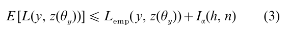
where I is the confidence interval, α is the alpha level of inferential statistics, and h is a quantity known as the Vapnik–Chervonenkis (VC) dimension (Vapnik and Chervonenkis 1971). The model that provides the lowest value of the upper bound for the expected risk should be chosen.

The VC dimension for a given model family of classification functions is defined as the maximum number of distinct binary samples that the model can fit perfectly without error for all possible labelings of the samples. Thus the VC dimension may be viewed as a measure of the complexity or flexibility of a model. Interestingly, the VC dimension depends not only on the number of parameters of a model but also, importantly, on the functional form of the model equation. A model with only one parameter can have infinite VC dimension while a model with a billion parameters can have a low VC dimension. For linear models, the VC dimension is equal to the number of parameters.

Given and n, the empirical risk L_emp( y, z(θ_y)) is a monotonically decreasing function of the VC dimension whereas the confidence interval I(h, n) is a monotonically increasing function of the VC dimension. These relationships along with the above equation reveal how structural risk minimization works. Among a set of competing models, the method chooses the model that describes the data sufficiently well (i.e., smallest empirical risk) with the least complex structure (i.e., narrowest confidence interval), thereby formalizing the principle of Occam’s razor. In practice, structural risk minimization is implemented by first creating a set of k nested models with successively increasing VC dimensions, h₁ < h₂ < …,< k, and then calculating the empirical risk for each model given sample data. The model with the smallest expected risk is then selected.

3.2 Regularization Theory

Regularization theory’s solution for solving the ill-posed problem is to secure the uniqueness of the solution by requiring it to satisfy some secondary condition that embeds prior information or assumptions about the solution. The form of prior information most often used is the condition that the unknown function being sought is sufficiently smooth. Formally, the regularization risk for a model is defined as

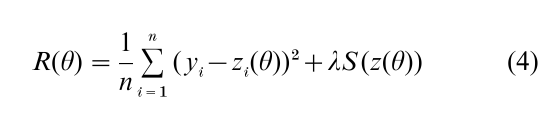
where the vector z(θ) is the model’s prediction at θ, is known as the regularization parameter, and S(z) is a functional that measures smoothness of the solution. The quantity often used for S(z) is the integral of the squared second derivatives with respect to an in-dependent variable x on which smoothness of the solution is assessed, i.e.,

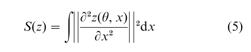
The regularization theory prescribes that the model with the smallest R(θ) should be chosen.

The first term of the above equation is a measure of the discrepancy between the data and the model’s prediction, that is, the empirical risk of the model. The second term, S(z), is a measure of complexity of the model. The larger the value of S(z), the less smooth theprediction,andthusthemorecomplexthemodel.The regularization parameter λ represents the relative importance of the complexity of the model with respect to its empirical risk. With λ₀ , the solution is primarily determined by observed data and thus tends to be highly complex in structure. On the other hand, with λ →∞, the smoothness condition entirely dictates the form of the solution, which tends to be simple in structure. In practice, a value between these two extremes is chosen based on some principled approach (Haykin 1999). In short, the regularization method, like the structural minimization method, uses complexity to steer the solution toward improved generalization. As such, it is another implementation of the principle of Occam’s razor.

3.3 Minimum Description Length

Minimum description length (MDL), which originated from algorithmic coding theory in computer science, regards both model and data as codes. The idea is that any data set can be appropriately encoded with the help of a model, and that the more we compress the data by extracting redundancy from it, the more we uncover underlying regularities in the data. Thus, code length is directly related to the generalization capability of the model, where the model that provides the shortest description of the data should be chosen. Formally, the total description length of a model is given by

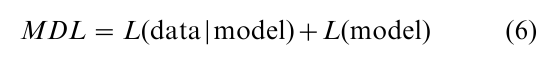
where L(data model) is the description length of the data given the model, measured in bits of information, and L(model) is the description length of the model itself.

The above definition of minimum description length is broad enough to be applied to any well-defined models, even verbally defined, qualitative models. For a statistical model defined as a parametrized family of probability distributions, the minimum description length for such a model takes the following form (Rissanen 1996):

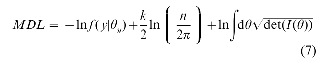
In the equation θ_y is the parameter value that maximizes the likelihood function f( y|θ), k is the number of parameters, I(θ) is the Fisher information matrix and det(I ) is the determinant of the matrix. The first term of the MDL can be interpreted as a measure of risk or lack of fit, and the second and third terms together are a measure of model complexity. Model evaluation is therefore carried out by trading off lack of fit for simplicity.

In summary, although the three approaches to model evaluation evolved from different conceptual frameworks and philosophies, they all share the common goal of achieving optimum generalizability by striking a balance between risk (or lack of fit) and complexity. Another commonality between these approaches is the aspect of a model that is captured by the complexity measure; they not only include the number of parameters in the model, but also, importantly, its functional form, which refers to the way in which the parameters are combined in the model equation.

4. Relations To Statistical Approaches

So far we have considered computational approaches that view model evaluation as an inductive inference problem, which is the predominant view in computer science and engineering. Model evaluation is also a topic of central interest for statisticians (statisticians prefer the term model selection to model evaluation). Approaches which have been developed within the statistical framework include the generalized likelihood ratio test (GLRT), cross-validation, the Akaike information criterion (AIC), the Bayesian information criterion (BIC) and Bayesian model selection. There are many important differences between these methods, but in essence, they all implement a means of finding, explicitly or implicitly, the best compromise between lack of fit and complexity by trading off one for the other. Statistical model selection methods are entirely consistent with the computational modeling approaches discussed above (see Sect. 3).

Here are a few notable differences and similarities between some of the statistical methods and computational methods. First, GLRT, AIC, and BIC differ from the computational methods such as structural risk minimization and minimum description length in that the two statistical selection criteria consider only the number of parameters as a complexity measure, and thus are insensitive to functional form, which can significantly influence generalizability. Second, application of the statistical methods requires that each model under investigation be a quantitative model defined as a parametric family of probability distributions. On the other hand, the computational methods can be applied to qualitative models as well as quantitative ones. For instance, the minimum description length method defined in Eqn. (4) is applicable to evaluating the effectiveness of decision tree models or even verbal models (Li and Vitanyi 1997). Finally, there exists a close connection between Bayesian model selection and the minimum description length criterion defined in Eqn. (5). The minimum description length criterion can be derived as an asymptotic approximation to the posterior probability in Bayesian model selection for a special form of the parameter prior density. An implication of this connection is that choosing the model that gives the shortest explanation for the observed data is essentially equivalent to choosing the model that is most likely to be true in the sense of probability theory (Li and Vitanyi 1997).

5. Conclusion

The question of how one should decide among competing explanations (i.e., models) of data is at the core of the scientific endeavor. A number of criteria have been proposed for model evaluation (Jacobs and Grainger 1994). They include (a) falsifiability: are there potential outcomes inconsistent with the model? (b) explanatory adequacy: is the explanation compatible with established findings? (c) interpretability: does the model make sense? Is it understandable? (d) descriptive adequacy: does the model provide a good description of the observed data? (e) simplicity: does the model describe the phenomenon in the simplest possible manner? and (f) generalizability: does the model predict well the characteristics of new, as yet unseen, data?

Among these criteria, computational modeling approaches described in this research paper, as well as statistical approaches, consider the last three as they are easier to quantify than the other three. In particular, generalizability has been emphasized as the principal criterion by which the effectiveness of a model be judged. Obviously, this ‘bias’ toward the predictive inference aspect of modeling reflects the dominant thinking of the current scientific community. Clearly one could develop an alternative approach that stresses other criteria, and even incorporates some of the hard-to-quantify criteria. There are plenty of opportunities in this area for the emerging field of model evaluation to grow and mature in the decades to come.

Bibliography:

1. Cherkassky V, Mulier F 1998 Learning from Data. Wiley, New York, Chaps. 2–4
2. Geman S, Binenstock E, Doursat R 1992 Neural networks and the bias-variance dilemma. Neural Computation 4: 1–58
3. Jacobs A M, Grainger J 1994 Models of visual word recognition-sampling the state of the art. Journal of Experimental Psychology: Human Perception and Performance 20: 1311–34
4. Haykin S 1999 Neural Networks: A Comprehensive Foundation. Prentice Hall, London, Chaps. 2, 4 and 5
5. Li M, Vitanyi P 1997 An Introduction to Kolmogoro Complexity and its Applications. Springer, New York
6. Rissanen J 1989 Stochastic Complexity in Statistical Inquiry. World Scientific, Singapore
7. Rissanen J 1996 Fisher information and stochastic complexity. IEEE Transaction on Information Theory 42: 40–7
8. Tikhonov A N 1963 On solving incorrectly posed problems and method of regularization. Doklady Akademii Nauk USSR 151: 501–4
9. Vapnik V N 1992 Principles of risk minimization for learning theory. Advances in Neural Information Processing Systems 4: 831–8
10. Vapnik V N, Chervonenkis A Y 1971 On the uniform convergence of relative frequencies of events to their probabilities. Theoretical Probability and Its Applications 17: 264–80