Structure Of Evolutionary Theory Research Paper

The theory itself represents the behavior of the system in terms of its states: the rules or laws of the theory (i.e., laws of coexistence, succession, or interaction) can delineate various configurations and trajectories on the state space. A description of the structure of the theory itself therefore only involves the description of the set of models, which make up the theory.

Construction of a model within the theory involves assignment of a location in the state space of the theory to a system of the kind defined by the theory. Potentially, there are many kinds of systems that a given theory can be used to describe—limitations come from the dynamical sufficiency (whether it can be used to describe the system accurately and completely) and the accuracy and effectiveness of the laws used to describe the system and its changes. Thus, there are two main aspects to defining a model. First, the state space must be defined—this involves choosing the variables and parameters with which the system will be described; second, coexistence laws, which describe the structure of the system and laws of succession, which describe changes in its structure, must be defined.

Defining the state space involves defining the set of all the states the system could possibly exhibit. Certain mathematical entities—in the case of many evolutionary models, these are vectors—are chosen to represent these states. The collection of all the possible values for each variable assigned a place in the vector is the state space of the system. The system and its states can have a geometrical interpretation: the variables used in the state description (i.e., state variables) can be conceived as the axes of a Cartesian space. The state of the system at any time may be represented as a point in that space, located by projection on the various axes.

The family of measurable physical magnitudes, in terms of which a given system is defined, also includes a set of parameters. Parameters are values that are not themselves a function of the state of the system. Thus, a parameter can be understood as a fixed value of a variable in the state space—topologically, setting a parameter amounts to limiting the number of possible structures in the state space by reducing the dimensionality of the model.

Laws, used to describe the behavior of the system in question, must also be defined in a description of a model or set of models. Laws have various forms: in general, coexistence laws describe the possible states of the system, while laws of succession describe changes in the state of the system.

Let us discuss in more detail the description of the evolutionary models that make up evolutionary theory. The main items needed for this description are the definition of a state space, state variables, parameters, and a set of laws of succession and coexistence for the system. Choosing a ‘state space’ (and thereby, a set of state variables) for the representation of genetic states and changes in a population is a crucial part of population genetics theory.

Paul Thompson suggests that the state space for population genetics would include the physically possible states of populations in terms of genotype frequencies. The state space would be ‘a Cartesian n- space where ‘n’ is a function of the number of possible pairs of alleles in the population’ (Thompson 1983 p. 223). We can picture this geometrically as n axes, the values of which are frequencies of the genotype. The state variables are the frequencies for each genotype. Note that this is a one-locus system; that is, we take only a single gene locus and determine the dimensionality of the model as a function of the number of alleles at that single locus.

Another type of single locus system, used less commonly than the one described by Thompson, involves using single gene frequencies, rather than genotype frequencies, as state variables. Some of the debates about ‘genic selectionism’ center around the adequacy of this state space and its parameters for representing evolutionary phenomena (see Lloyd 1988/1994, Chap. 7). With both genotype and gene frequency state spaces though, treating the genetic system of an organism as being able to be isolated into single loci involves a number of assumptions about the system as a whole. For instance, if the relative finesses of the genotypes at a locus are dependent on other loci, then the frequencies of a single locus observed in isolation will not be sufficient to determine the actual genotype frequencies. Assumptions about the structure of the system as a whole can thus be incorporated into the state space in order to reduce its dimensionality. Lewontin (1974) offers a detailed analysis of the quantitative effects of dimensionality of various assumptions about the biological systems being modeled.

Interactions between genotypes, and between one locus and another cannot be represented in a single locus model (with the exception of frequency-dependent selection), for the simple reason that they involve more than one locus (Lewontin 1974, pp. 273–81, Wimsatt 1980, pp. 226–9).

Although all single locus models should, in some sense, be grouped together, they are not all exactly the same model—each particular model has a different number of state variables, depending upon the number of alleles at that locus. Bas Van Fraassen suggests calling the general outline for each model its ‘model type’ (1980, p. 44). Because a model type is simply an abstraction of a model, constructed by abstracting one or more of the models parameters, a single model can be an instance of more than one model type.

Along similar lines, we may say that each model type be associated with a distinctive state space type. In the preceding example, the single locus model is to be taken as an instance of a general state space type for all single locus models, i.e., the different single locus model types are conceived as utilizing the same state space type. Alternatives, such as two-locus models, must be taken as instances of a different state space type.

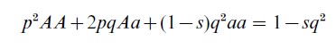
‘Parameters’ are the values that appear in the succession and coexistence laws of a system that are the same for all possible states of the defined system. For instance, in the modification of the Hardy– Weinberg equation that predicts the frequencies of the genotypes after selection, the selection coefficient, s, appears as a parameter in the formula

There are a variety of methods of establishing the value at which a parameter should be fixed or set in the construction of models for a given real system, e.g., simulation techniques can be used to obtain estimates of biologically important parameters. In some contexts, maximum likelihood estimations may be possible. Parameters can also be set arbitrarily, or ignored. This is equivalent to incorporating certain assumptions into the model for purposes of simplification (Levins 1968, pp. 8, 89).

One expects the values of parameters to have an impact on the system being represented; but variations in parameter values can make a larger or smaller amount of difference to the system. For instance, take a deterministic model that incorporates a parameter for mutation, µ. The rates of change of this model are virtually insensitive to realistic variations in the value of µ. Yet the selection parameters play a crucial role in this same model. A very small amount of selection in favor of an allele will have a cumulative effect strong enough to replace other alleles (Lewontin 1974, p. 267).

Population size is another case in which the value assigned to the parameter has a large impact on the model results. The parameter for effective population size, N, can play a crucial role in some models, because selection results can be quite different with a restricted gene pool size (Mayr 1967, pp. 48–50). In many of the stochastic models involved in calculating rates of evolutionary change, the resulting distributions and their moments can depend completely on the ratio of the mean deterministic force to the variance arising from random processes (Lewontin 1974, p. 268). This variance is usually proportional to 1/N and is related to the finiteness of population size. Thus, change in the value of the single parameter, N, can completely alter the structure represented by the theory.

The choice of parameters can also make a major difference to the model outcome. Theoreticians have choices about how to express certain aspects of the system or environment. The choice of parameters used to represent the various aspects can have a profound effect on the structure, even to the point of rendering the model useless for representing the empirical system in question. Group selection models provide a case in which choice of parameters not only alters the results of the models, but also leads to the near disappearance of the phenomenon being modeled (Wade 1978).

Some authors, when discussing genetic changes in populations, speak of the system in terms of a phenotype state space type. This makes sense, because the phenotype determines the breeding system and the action of natural selection, the results of which are reflected in the genetic changes in the population. In his analysis of the present structure of population genetics theory, Lewontin traces a single calculation of a change in genetic state through both genotypic and phenotypic descriptions of the population. That is, according to Lewontin, population genetics theory must map the set of genotypes onto the set of phenotypes, give transformations in the phenotype space, and then map the set of phenotypes back onto the set of genotypes. We would expect, then, that descriptions of state in population genetics would be framed in terms of both genotypic and phenotypic variables and parameters. But this is not the case—the description can be in terms of either genotypic or phenotypic variables, but not both. Dynamically, then, it seems as if population genetics must operate in two parallel systems: one in genotype state space, one in phenotype state space (Lewontin 1974).

Lewontin explains that such independence of systems is illusory ‘and arises from a bit of sleight-ofhand in which phenotype and genotype variables are made to appear as merely parameters that need to be experimentally determined, constants that are not themselves transformed by the evolutionary process’ (1974, p. 15).

Now consider a few particular aspects and forms of the ‘laws’ used in these models. The most obvious differences, in laws as well as in state space types, are between deterministic and stochastic models. Coexistence laws describe the possible states of the system in terms of the state space. In the case of evolutionary theory, these laws would consist of conditions delineating a subset of the state space that contains only the biologically possible states. Laws of succession describe changes in the state of the system. In the case of evolutionary theory, dynamic laws concern changes in the genetic composition of populations.

The laws of succession select the biologically possible trajectories in the state space, with states at particular times being represented by points in the state space. The law of succession is the equation of which the biologically possible trajectories are the solutions. The Hardy–Weinberg equation is the fundamental law of both coexistence and succession in population genetics theory. Even the dynamic laws of the theory are usually used to assess the properties of the equilibrium states and steady state distributions. The Hardy–Weinberg law is a very simple, deterministic succession law that is used in a very simple state space. As parameters are added to the equation, we get different laws, technically speaking. For example, compare the laws used to calculate the frequency p of the A allele in the next generation. Plugging only the selection coefficient against a recessive into the basic Hardy–Weinberg law, we get the recursion for the dominant allele frequency as p`=p/(1-sq<sup>2</sup>). Addition of parameters for the mutation rates yields a completely different law, p“=1-µp`+νq`, where µ is the rate of mutation away from the dominant allele, and where ν is the rate of mutation towards it. We could consider these laws to be of a single type— variations on the basic Hardy–Weinberg law—which are usually used in a certain state space type. The actual state space used in each instance depends on the genetic characteristics of the natural system, and not usually on the parameters. For instance, the succession of a system at Hardy–Weinberg equilibrium and one that is not at equilibrium but is under selection pressure, could both be modeled in the same state space, using different laws.

A theory can have either deterministic or statistical laws for its state transitions. Furthermore, the states themselves can be either statistical or non-statistical. In population genetics models, gene frequencies that often appear in the set of state variables, thus the states themselves are statistical entities. In general, a law is deterministic if, when all of the parameters and variables are specified, the succeeding states are uniquely determined. In population genetics, this means that the initial population and parameters are all that is needed to get an exact prediction of the new population state.

In sum, the structure of evolutionary theory can be understood by examining the family of models it presents. In the case of population genetics theory, the set of model types—stochastic and deterministic, single locus or multilocus—can be understood as a related family of models. The question then becomes defining the exact nature of the relationships among them.

2. Confirming And Testing Models

The most obvious way to support a claim of the form ‘this natural system is described by this model,’ is to demonstrate the simple matching of some part of the model with some part of the natural system being described. For instance, in a population genetics model, the solution of an equation might yield a single genotype frequency value. The genotype frequency is a state variable in the model. Given a certain set of input variables (e.g., the initial genotype frequency value, in this case), the output values of variables can be calculated using the rules or laws of the model. The output set of variables (i.e., the solution of the model equation given the input values of the variables) is the ‘outcome’ of the model. Determining the fit between model and natural system involves testing how well the genotype frequency trajectory calculated from the model (the outcome of the model) matches that measured in the relevant natural (or experimental) populations. It can be evaluated by determining the fit of one curve (the model trajectory or coexistence conditions) to another (taken from the natural system); ordinary statistical techniques of evaluating curve-fitting are used.

Also, numerous assumptions are made in the construction of any model, and testing a model sometimes involves confirming some or all of these assumptions independently. These include assumptions about which factors influence the changes in the system, what the ranges for the parameters are, and what the mathematical form of the laws is. On the basis of these assumptions, the models take on certain features. Many of these assumptions thus have potential empirical content. That is, although they are assumptions made about certain mathematical entities and processes during the construction of the theoretical model, when empirical claims are then made about this model, the assumptions may have empirical significance.

For instance, the assumption might be made during the construction of a model that the population is panmictic, i.e., that all genotypes interbreed at random with each other. The model outcome, in this case, is still a genotype frequency trajectory, for which ordinary curve-fitting tests can be performed on the natural population to which the model is applied. But the model can have additional empirical significance, given the empirical claim that a natural system is a system of the kind described in the model. The assumption of panmixia, as a description of the population structure of the system under question, must be considered part of the system description that is being evaluated empirically. Evidence to the effect that certain genotypes in the population breed exclusively with each other (i.e., evidence that the population is not, in fact, panmictic) would undermine empirical claims about the model as a whole, other things being equal, and even if genotype frequencies provide good instances of fit. In other words, the assumption that genotypes are randomly redistributed in each generation is intrinsic to many population genetics model types. Hence, although the assumption that the population is panmictic often is taken for granted in the actual definition of the model type—i.e., in the law formula—it is interpreted empirically and plays an important role in determining the empirical adequacy of the claim.

By the same token, evidence that the assumptions of the model hold for the natural system being considered will increase the credibility of the claim that the model accurately describes the natural system. Technically, we can describe this situation as follows. From the point of view of empirical claims made about it, the model has three parts: state variables, empirically interpreted background assumptions, and those aspects and assumptions of the model that are not directly empirically interpreted. Because the possible outcomes of the model (along with the inputs) are actually values of the state variables, we can understand the input and outcome of the model as a sort of minimal empirical description of the natural system. If a model is claimed to describe accurately a natural system, at the very least, this means that the variables in which the natural system is described change according to the laws presented in the theoretical model. Under many circumstances, such models, in which only the state variables are empirically interpreted, are understood to be ‘mere’ calculating devices, because the isomorphism with the natural system is so limited.

Moreover, various aspects of the model—for instance, the form of its laws, or the values of its parameters—rely on assumptions made during model construction that can be interpreted empirically. The assumption of panmixia, discussed above, is an empirically interpreted background assumption of many population genetics models. Because it is empirically interpreted, the presence or absence of panmixia in the natural population in question makes a difference to the empirical adequacy of the model.

Finally, there may be aspects of the model that are not interpreted empirically at all. For instance, some parameters appearing in the laws might be theoretically determined and might have no counterpart in the natural system against which the model is compared.

Given that there can be aspects of the model structure that are not directly tested by examining the fit of the state variable curve, direct testing of these other aspects would give additional reason to accept (or reject) the model as a whole. In other words, it is taken that direct testing provides a stronger test than indirect testing, hence there is a higher degree of confirmation if the test is supported by empirical evidence. Direct empirical evidence for certain empirically interpreted aspects of the model that are not included in the state variables (and thus are confirmed only indirectly by goodness-of-fit tests), therefore provides additional support for the application of the model.

The above sort of testing of assumptions involves making sure that the empirical conditions for application of various parts of the model description actually do hold. In other words, in order to accept an explanation constructed by applying the model, the conditions for application must be verified. The specific values inserted as the parameters or fixed values of the model are another important aspect of empirical claims that can be tested. In some models, mutation rates, etc., appear in the equation—part of the task of confirming the application of the model involves making sure that the values inserted for the parameters are appropriate for the natural system being described. Finally, there is a more abstract form of independent support available, in which some general aspect of the model, for instance, the interrelation between the two variables, or the significance of a particular parameter or variable, can be supported through evidence outside the application of the model itself.

Lastly, variety of evidence, of which there are three kinds, is an important factor in the evaluation of empirical claims. I discuss three kinds of variety of evidence here: (a) variety of instances of fit; (b) variety of independently supported model assumptions; and (c) variety of types of support, which include fit and independent support of aspects of the model.

First, let us consider variety of fit, that is, variety of instances in which the model outcome matches the value obtained from the natural system. Traditionally, variety of evidence has meant variety of fit. There are two issues that must be distinguished when considering the variety of fit. One involves the range of application of a model or model type, while the other involves the degree of empirical support provided for a single application. Both of these issues involve the notion of independence, which needs to be clarified before continuing.

One point of any claim to variety of evidence is to show that there is evidence for the hypothesis in question from different or independent sources. The notion of independence here is problematic. It is not the sort of independence that is found in the frequency interpretation of probability theory, where the independence depends only on accepting a particular reference class. Rather, in the context of scientific theories, independence is relative to whatever theories have already been accepted.

In evolutionary theory, independence is usually relative to some assumption about natural kinds. Often, empirical claims are made to the effect that a model is applicable over a certain range of natural systems. Inherent in these claims is the assumption that all of the natural systems in the range participate in some key feature or features that make it possible and/or desirable to describe them all with the same model type. Thus, there is some assumption of a natural kind (characterized by the key feature or features) whenever range of applications arises. The scientist, in making a claim that the model type is applicable to such and such systems, is making an empirical assumption about the existence of the key feature or features in the range of natural systems under question. Hence, for evolutionary models, testing for variety of fit depends on accepting an assumption about what constitutes different or independent instances of fit; this in turn, amounts to accepting a particular view of natural kinds. Part of what variety of evidence does, in a bootstrapping effect, is to confirm this original assumption about natural kinds. More technically, variety of evidence confirms the sufficiency of the parameters and state space.

Take the case in which a model type is claimed to be applicable over a more extended range than that actually covered by available evidence. This extrapolation of the range of a model can be performed by simply accepting or assuming the applicability of the model to the entire range in question. A more convincing way to extend applicability is to offer evidence of fit between the model and the data in the new part of the range. Provision of a variety of fit can thus provide additional reason for accepting the empirical claim regarding the range of applicability of the model.

For instance, a theory confirmed by ten instances of fit involving populations of size 1,000 (where population size is a relevant parameter) is in a different situation with regard to confirmation than a theory confirmed by one instance of each of ten different population sizes ranging from 1 to 1,000,000. If the empirical claims made about these two models asserted the same broad range of applicability, the latter model is confirmed by a greater variety of instances of fit. That is, the empirical claim about the latter model is better confirmed, through successful application (fits) over a larger section of the relevant range than the first model. Variety of fit can therefore provide additional reason for accepting an empirical claim about the range of applicability of a model. Variety of fit can also provide additional reason for accepting a particular empirical claim, i.e., one of the form, ‘this natural system is accurately described by that model.’ That is, variety of evidence can serve to increase confidence in the accuracy of any particular description of a natural system by a model.

Variety of fit is only one kind of variety of evidence. An increase in the number and kind of assumptions tested independently, i.e., greater variety of assumptions tested, would also provide additional reason for accepting an empirical claim about a model. The final sort of variety of evidence involves the mixture of instances of fit and instances of independently tested aspects of the model. In this case, the variety of types of evidence offered for an empirical claim about a model is an aspect of confirmation.

According to the view of confirmation sketched above, claims about models may be confirmed in three different ways: (a) through fit of the outcome of the model to a natural system; (b) through independent testing of assumptions of the model, including parameters and parameter ranges; and (c) through a range of instances of fit over a variety of the natural systems to be accounted for by the model, through a variety of assumptions tested, and including both instances of fit and some independent support for aspects of the model.

Bibliography:

1. Levins R 1968 Evolution in Changing Environments. Princeton University Press, Princeton, NJ
2. Lewontin R C 1974 The Genetic Basis of Evolutionary Change. Columbia University Press, New York
3. Lloyd E A 1988/1994 The Structure and Confirmation of Evolutionary Theory. Princeton University Press, Princeton, NJ
4. Mayr E 1967 Evolutionary challenges to the mathematical interpretation of evolution. In: Moorehead P S, Kaplan M M (eds.) Mathematical Challenges to the Neo-Darwinian Interpretation of Evolution. Wistar Institute Press, Philadelphia, pp. 47–54
5. Thompson P 1983 The structure of evolutionary theory: A semantic perspective. Studies in History and Philosophy of Science 37: 215–29
6. Van Fraassen B C 1980 The Scientific Image. Clarendon Press, Oxford University Press, Oxford, UK
7. Wade M 1978 A critical review of the models of group selection. Quarterly Review of Biology 53: 101–14
8. Wimsatt W 1980 Reductionist research strategies and their biases in the units of selection controversy. In: Nickles T (ed.) Scientific DiscOvery: Case Studies. Reidel, Dordrecht, The Netherlands, pp. 213–59