Comparative Method in Evolutionary Studies Research Paper

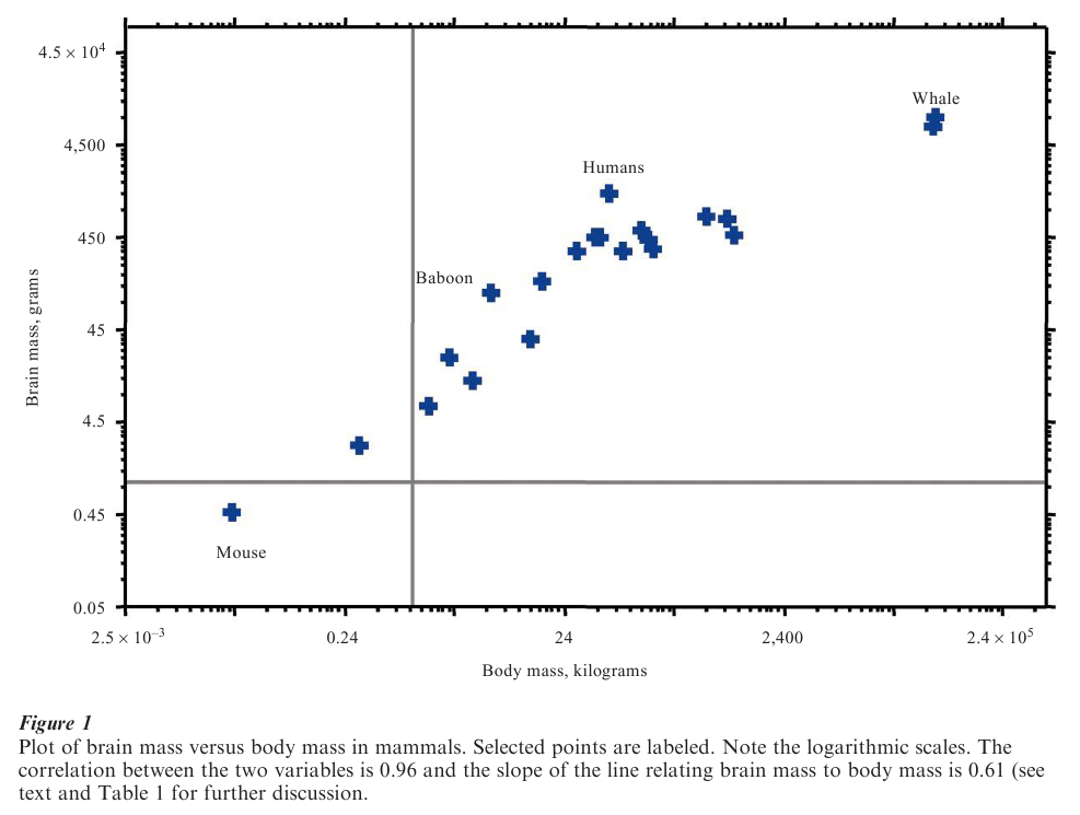
One of the classic comparative relationships is that between the size of an organism’s body and the size of its brain (Fig. 1): brain size increases steadily and predictably with body size in mammals, and this relationship also holds within most other animal groups. Much of the interest that comparative relationships such as this one generate derives from their ability to reveal broad or general evolutionary trends. Table 1 lists a small number of such trends and the species in which they have been found.

Comparative trends, in addition to describing the ‘end-points’ of evolution across contemporary species, can also be shown to have an historical interpretation: the relationship observed across a group of con- temporary or extant species reflects the correlation that would have held in the ancestral species as they evolved over time up to the present (Pagel 1993). Thus, the relationships reported in Table 1 tell us that as organisms evolve and grow larger, their lifespan, ages at maturity, brain size, and basal metabolic rates increase, but their heart rates slow down.

The natural interpretation of comparative relationships is that they reveal adaptive trends. This is to say that the organisms that individually evolved to produce the trend were somehow more fit or suited for survival than those that did not. Thus, as animals evolve to become larger, a larger brain is required for ‘housekeeping’ functions as well as simply to monitor the increased number of neuronal signals coming from the organism’s body and internal organs. Larger animals also tend to roam over wider areas and a larger brain may be advantageous for taking ad-vantage of what the terrain has to offer. Small animals could have larger brains, but if the adaptive argument is correct, a relatively large brain in a small animal might be a disadvantage. Brains are costly to produce and maintain (they must be supplied with blood and nutrients) and so animals are unlikely to evolve ‘spare capacity.’

Some comparative trends reveal a relationship that is mediated by some other set of factors. It is not obvious why a longer lifespan is only advantageous to larger animals. Would not a small organism benefit from living a long time and thereby having more opportunity to reproduce? One possibility is that smaller organisms suffer higher rates of mortality, from natural variation in the environment to higher rates of predation. If this is true, it may not pay smaller organisms to evolve to have a long lifespan. Rather, natural selection may favour adaptations in small organisms that allow them to grow, mature, and reproduce rapidly: there is little point in a ‘slow and steady’ lifestyle if one is likely to be dead before reaching maturity. Conversely, a slow and steady lifestyle may be advantageous to longer-lived species. By putting resources into producing a large and healthy body, an individual may be able to produce a larger number of offspring over a long period of time.

When such additional factors are thought either to mediate a relationship or to offer an alternative explanation, comparative methods can still be applied. The relationship between two variables can be investigated, having statistically removed the effects of a third. Rates of mortality, for example, remain correlated with lifespan even after controlling for body size: thus, one can say that decreasing mortality rates, for a given body size, will be associated with a longer lifespan. These examples show that comparative studies can both test adaptive hypotheses and reveal trends whose precise causes can often be discovered by further investigation. Alternatively, a comparative trend might be regarded as evidence, not of adaptation, but rather of some form of constraint. Animals with larger bodies may have larger brains because the genes that make larger bodies also make larger brains. Similarly, larger animals may have a longer lifespan simply because it takes longer to grow a larger body than a small one. This tension between adaptive and nonadaptive explanations for observed comparative trends is what drives investigators to make ever more precise tests of their hypotheses. So-called nonadaptive hypotheses can often be tested by controlling for suitable ‘third’ variables.

1. The Problem Of Independence

One of the strongest pieces of evidence that a comparative relationship represents an adaptive trend is to show that it has arisen independently on more than one occasion. Were this simply a matter of collecting information on a wide range of species and plotting a trend, the ‘comparative method’ would be little more than a commonsense set of rules for displaying information. However, the hierarchical nature of biological evolution means that individual species can seldom be considered independent instances of the adaptive relationship.

Over evolutionary time species evolve and give rise to daughter species which in turn give rise to more species. At each branching point in evolution, the ancestral species may live on independently of its daughter species, or it and its daughter species may evolve into something slightly different from the ancestral form. The collection of such ancestral-descendant relationships among a set of species is described by a phylogenetic tree. Phylogenetic trees are characterized by a series of branching points leading from the ‘root’ or common ancestor of the species up to the tips or contemporary organisms.

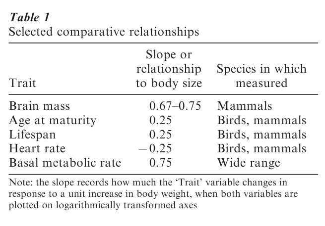
The phylogenetic tree diagram also makes clear why species cannot typically be considered independent instances of an adaptive trend. Consider the example of Fig. 2(a). Eight species, all descendant from a common ancestor take the values A, B on two traits. Eight other species, all descendant from a different common ancestor, take the values a, b on the same traits. The relationship counted across the sixteen species is perfect: ‘A’ always goes with ‘B’ and ‘a’ always goes with ‘b.’ But the phylogeny of these sixteen species reveals that the pairing A, B and a, b probably arose only once. For sake of argument, assume that the ancestor at the root of the tree was {A, B} and that the traits ‘a’ and ‘b’ evolved along the branch leading to the ancestor to the eight species on the right of the diagram. These traits were then retained in the eight descendants.

The phylogenetic perspective forces us to realize that what might have appeared to be a broad adaptive trend linking two traits could be little more than a chance pairing. For some reason ‘a’ and ‘b’ each evolved in the same branch, but quite possibly in-dependently of each other. Their retention in the eight contemporary species is no evidence at all that they coevolve: each may be adaptive in its own right, but their joint presence is not evidence that they evolved together for some adaptive reason.

If the phylogenetic tree looked like that of Fig. 2(b), however, then there would be evidence that the relationship a, b had evolved repeatedly: that is, on a number of independent occasions, when ‘a’ evolved, so did ‘b.’ The summary of the number of species with traits {A, B} and a, b would be identical to that of Fig. 2(a). But, the result in Fig. 2(b) would compel us to seek evidence for a link between ‘a’ and ‘b’ in a way that was missing from Fig. 2(a).

These considerations lead to the following import-ant conclusion: the strength of evidence for an adaptive relationship in a comparative study derives, not from knowing how many species come to inherit some set of traits, but in how many times the relationship between two traits has arisen independently. Nearly all of the effort among researchers who design methods for comparative studies has been directed at this problem of independence and how to exploit phylogenies to reveal independent events of evolution.

2. Phylogenies And Independent Evolution: A Brief History

Three broad classes of method have been developed to identify independent events of evolution in phylogenies: so-called higher-nodes approaches, phylogenetic-subtraction techniques, and methods that partition the phylogeny into independent subsets of information. Of these three classes, those that partition the phylogeny came to be dominant. Very recently new statistical approaches have begun to replace these partitioning methods.

The higher-nodes approach seeks to identify a level of taxonomic classification that can be considered independent for statistical purposes and then restricts analysis to that level. For example, it is well established that in mammals, most of the diversity in brain and body size observed across species, is evident in differences among taxonomic ‘orders’ and ‘families.’ The Carnivora are an example of a Mammalian order and within the Carnivora the family felidae comprises the cats. The Artiodactyls and the bo idae (the cows) are another example of an order and family. Orders and families are commonly referred to as ‘higher’ taxonomic levels. In this instance, the higher nodes approach would proceed by analyzing differences among family means and counting families—not species—as the independent units of analysis. This would be analogous in Fig. 2(a) to comparing only the two nodes of the phylogeny. Here the procedure works by suggesting that there are only two independent data points in the phylogenetic tree, properly recognizing that the differences represented among the sixteen species arose independently perhaps only once.

Phylogenetic-subtraction methods proceed in a manner directly opposite to the higher-nodes in their attempts to identify independent evolution. These approaches seek to identify variation among species that is independent of their phylogenetic relationships to each other. Thus, taking again the example of brain and body size, the phylogenetic subtraction methods would subtract the appropriate taxonomic family-mean from each species data point. The resulting ‘residual’ value is taken to represent evolution that is independent of that species phylogenetic position. Applied to Fig. 2(a), the phylogenetic-subtraction methods would calculate the mean values at each of the two nodes, then subtract the appropriate mean from each species. Here the phylogenetic-subtraction methods would identify that none of the variability among species was independent of the immediately ancestral nodes.

Both the higher-nodes and phylogenetic-subtraction methods remove some portion of the variability among the species in an attempt to identify independent examples of evolutionary change among species. The successor to both of these classes of approach, partitioning methods, was based upon the recognition that the phylogeny itself provides a way of partitioning all of the variability amongst species into a set of, in principle, independent units of evolution. That is, none of the variability is discarded.

The best known partitioning method is that of independent-contrasts. A contrast is defined as a difference between two species, a species and a node of the phylogeny, or between two nodes. Careful choice of the contrasts yields a set of difference scores such that each member of the set is independent of each other member and which collectively account for all of the observed variability amongst species.

Figure 2(b) shows how the independent-contrast methods work. The phylogeny shows that species 1 and 2 share an immediate common ancestor. Thus, the simple numerical difference between these two species on the trait of interest identifies some amount of evolution that occurred since they branched from their common ancestor. Similarly, differences among other pairs of species identify amounts of evolution that arose since they diverged from their common ancestor and which are independent of the other pairs of species in the phylogeny. The phylogeny identifies eight such differences among the tips of the tree. Moving back one level on the tree, four additional differences can be calculated, corresponding to pairs of nodes that immediately precede the tips of the tree. Each of these differences also measures a unique portion of the evolutionary change on the tree. Here, the comparisons reveal that no evolution has taken place on the traits between pairs of these more ancestral nodes. Moving back another level there are two more comparisons, and finally the last comparison, that between the nodes that represent the two descendants of the root or common ancestor of the whole tree.

In this manner, fifteen comparisons have been identified for the sixteen species. These fifteen comparisons, each one in principle independent of the others, exhaust the variability in the phylogeny, treating all of it as relevant to the hypothesis test. By comparison the phylogenetic-subtraction methods and the higher-nodes approaches always exclude some portion of the variability among the species’ traits. In general, with a bifurcating tree (each node gives rise to two descendants) such as seen in Fig. 2(b), there will always be n 1 independent contrasts, given n species.

A set of contrasts can be calculated separately for each of two or more traits, then the correlation of the two sets of contrasts is used to test the hypothesis of coevolution. Importantly, each pair of contrasts pro-vides an independent test of the hypothesis of coevolution: if, for example, brain size and body size covary, then each positive difference in body size between a pair of species (or nodes) should be accompanied by a positive difference in brain size. Further, larger differences in body size should be accompanied by larger differences in brain size.

3. New Statistical Methods And The Analysis Of Comparative Data

The capability of independent-contrasts methods to use all of the variability in the phylogeny made them the favored technique of comparative analysis throughout the 1990s. A new set of statistical methods based upon the statistical approach known as maxi-mum likelihood has since replaced these techniques. The new methods, like their predecessors, identify independent instances of evolution in the phylogeny. They do so without the mechanical procedure of forming contrasts or of calculating means at higher nodes and they have greater flexibility for manipulating the phylogeny and the species data. They also retain information that is lost in the independent-contrast approach. For example, contrast methods cannot estimate the ancestral state at the root of the phylogeny.

In words, the new methods use the phylogeny to specify the expected lack of independence among species. They then use that information to adjust the statistical analysis internally to reflect the lack of independence. The new methods have been developed for two broad classes of data: discrete or categorical variable methods are applied to data that fall into a small number (typically two) of discrete classes or categories. Diet type, mating system, and the presence or absence of some feature or behavior are examples of this kind of data. The statistical Markov-model provides a natural framework for discrete traits (Pagel 1994). Continuousariable methods are applied to traits that are measured on a continuous scale. Most traits relating to size, shape, timings, frequency, or concentrations are measured on continuous scales. For this kind of data a statistical technique known as generalized least squares or GLS is well suited to analyze trait evolution on a phylogeny (Garland 2000, Schluter et al. 1997, Martins and Hansen 1997, Pagel 1997, 1999)

3.1 Correlated Evolution Of Continuously Evolving Traits: The GLS Approach

The most commonly used model for continuously evolving traits is the constant-variance random-walk process (sometimes called Brownian-motion). In the conventional random-walk model, traits evolve each short instant of time dt by some random amount that might be positive (for example, the trait gets larger) or negative. The successive random changes to a trait are independent of each other, they have a mean or average of zero, an d some unknown and constant variance, denoted σ .

The random-walk is presumed to unfold independently at each instant of time and along each of the branches of the phylogeny. Given this, the phylogeny specifies how much a given species’ trait value is expected to vary were evolution to be rerun as a random walk many times (this is the variance, σ ), and how similar any pair of species are expected to be. These are the quantities that are needed to adjust the statistical analysis for nonindependence amongst species.

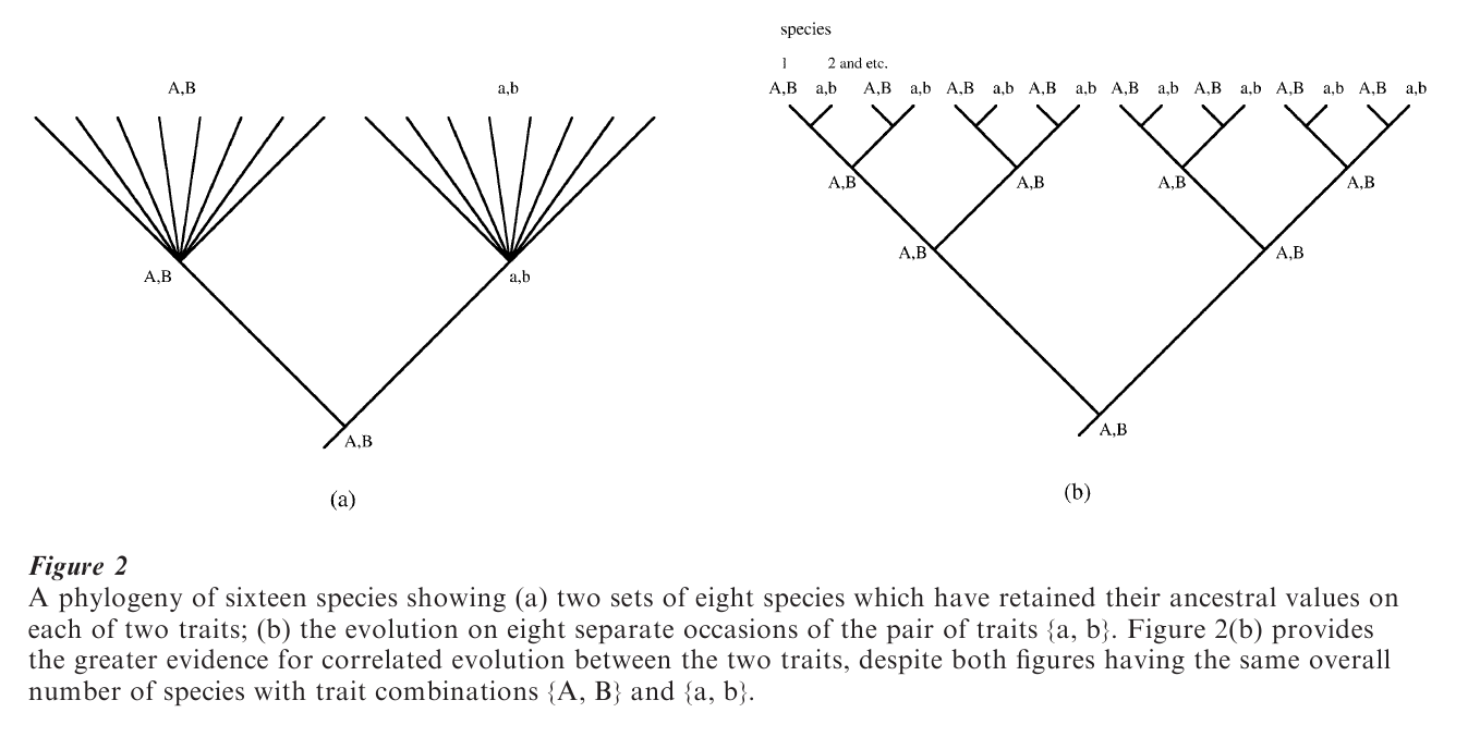
The variance of any species’ trait value turns out to be given by tσ², where t is the total path length from the root of the phylogeny to the species (the summation of all the small dts); t might be measured in units of time or in units of ‘operational time’ such as genetic divergence. Closely-related species will tend to have similar trait values, even under a random-walk, owing to sharing most of their evolutionary history. The expected covariance (like a correlation) between two species in their trait values is given by t_sσ² , where the subscript s denotes the shared path length from the root up to the point at which the two species separate.

The generalized least squares model represents the information about the expected variances and covariance of species in a matrix, usually denoted V. Figure 3 shows the matrix V that is implied by the simple phylogeny depicted there. GLS statistical methods use V to adjust internally for the expected lack of independence among species. This means that one can simply analyze the species data points as if they were independent, the nonindependence having been controlled for automatically by V. It also means that one can specify transformations of V that effectively change the underlying model of evolution (Pagel 1999).

3.2 Mammalian Brain-Size Evolution

The evolution of mammalian brain size provides a good example of the use of the GLS approach to analyze comparative data. Theories of the evolution of mammalian brain size link brain volume to body mass either through body surface area or through basal metabolic rate. The surface area hypothesis requires that the slope of the line relating brain volume to body mass is 2/3; the metabolic rate hypothesis predicts that the slope of brain volume against body mass will be 3/4, owing to the relationships of basal metabolic rate to body and brain size. Empirically derived brain-body slopes generally lie somewhere in the 2/3 to 3/4 range.

Applied to the data of Fig. 1 and using a suitable phylogeny of the mammals, the GLS model returns a slope relating brain mass to body mass of 0.61. This is lower than the expected 2/3 to 3/4, despite a very strong correlation between the two traits (Table 2). Even in these comparatively small samples, the 95% confidence intervals exclude 3 4, and nearly exclude 2/3. The GLS model also estimates the ancestral mammalian brain and body sizes, here found to be a brain mass of 20 grams and a body mass of about 5 kilograms. By comparison to the brain and body size relationship, the slope of basal metabolic rate to body mass (Table 2) is near to the expected value of 0.75 (Table 1).

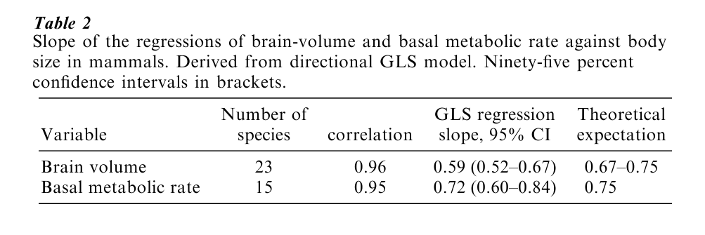
The GLS model returns unfavorable support for the surface-area and metabolic rate theories of mam-malian brain size. Theories linking brain-adaptations to specific environmental demands may offer new ways of thinking about brain evolution.

3.3 Testing The Adequacy Of The Model Of Evolution

The GLS approach makes it possible to test the adequacy of the underlying constant-variance (Brownian motion) model and to test hypotheses about trait evolution (Pagel 1999; see also Table 3). This is done by transforming the elements of V. A parameter κ scales individual phylogenetic branch lengths and can be used to test for a punctuational mode of evolution; a parameter δ scales overall path lengths in the phylogeny—the distance from the root to the species—and can detect adaptive radiations; and a parameter λ asks whether the phylogeny correctly predicts the patterns of variance and covariance. If species are evolving as if they are independent, this parameter will indicate that phylogenetic correction can be dispensed with, and will automatically do so.

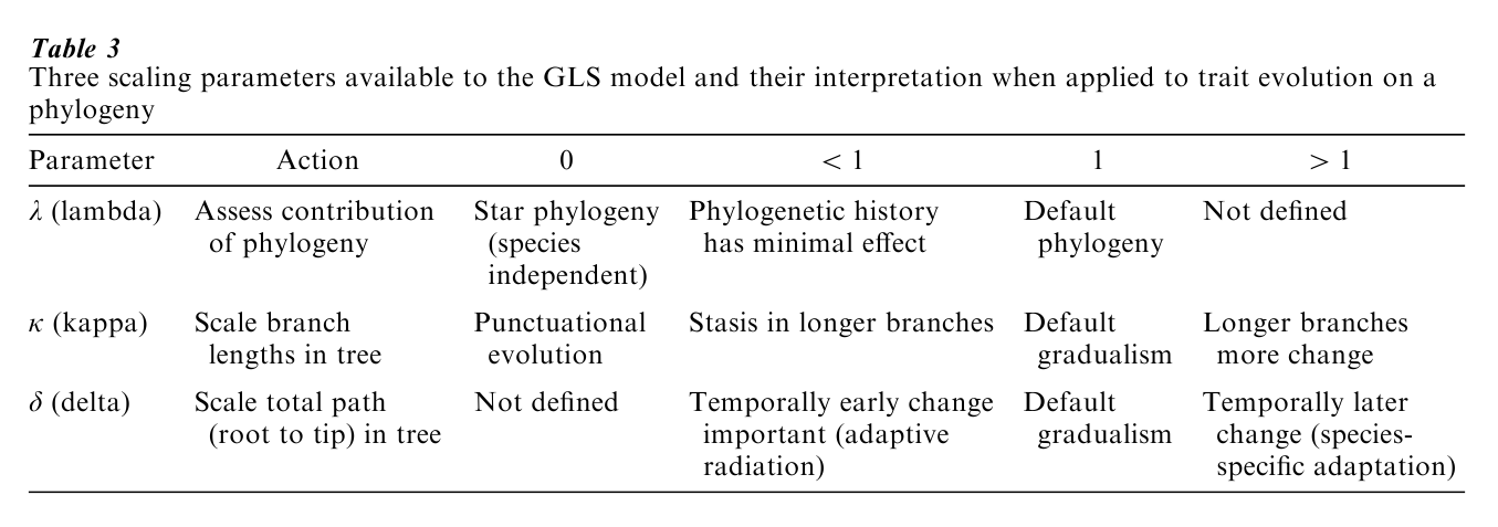
For the brain and body size data, the 95 percent confidence intervals of all three parameters overlap 1.0, the default values under the constant-variance model: κ=1.06 (0.42–1.63); δ=0.96 (0.078–2.79); and λ=1.0 (0.94–1.0). These values justify using the phylogeny to correct for nonindependence, and indicate that trait evolution is proportional to the branch lengths.

3.4 Correlated Evolution Of Discrete Traits: The Marko Model

The Markov-transition process is the statistical model widely used to describe the evolution of traits that adopt only a finite number of states. The Markov approach estimates the rates at which a trait or character makes transitions amongst its possible states as it evolves over time. A trait is assumed to begin some epoch of time in one of its possible states and then at each short epoch of time dt it can jump to one of its other states. The Markov transition rates are the rates at which these jumps are made. These rates are sufficient to calculate the most probable states at any node or tip of a phylogeny, given some starting point at the root. Similar to the situation with continuously evolving characters, closely related species will typically have similar trait values under a Markov model, whereas more distantly related species are not expected to be as similar.

To test for correlated evolution between two binary discrete characters the Markov model compares the fit of two models to the data. In one the two traits are allowed to evolve independently; in the other they evolve in a correlated fashion. Evidence for a correlation is found if the model of correlated evolution fits the data significantly better than the model of independent evolution (Pagel 1994).

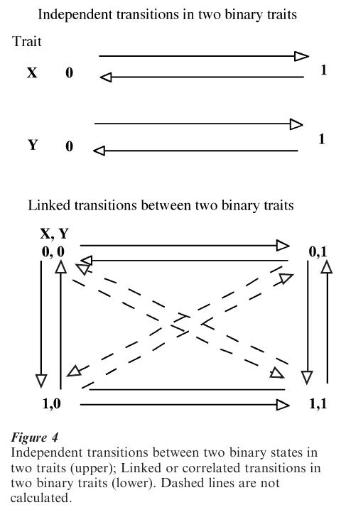
For a trait that can take only two values (e.g., 0,1), two rates must be estimated, one for transition from ‘0’ to ‘1,’ and the other for transitions from ‘1’ to ‘0.’ Four parameters are required for two traits evolving independently. The model of correlated evolution considers the four possible states that two binary characters can jointly adopt (0,0; 0,1; 1,0; 1,1). It then allows one of the variables to change state in any branch of the tree, yielding eight possible transitions to be estimated (Fig. 4). These can be shown to be sufficient to calculate the probability of any kind of change in any branch of the tree, and they can be used to chart the most probable course of evolution from the ancestral state to the contemporary derived state.

3.5 The Evolution Of Lactose-Tolerance

The evolution of lactose tolerance in human societies illustrates how to test for correlated evolution using two discrete traits. The lactase enzyme confers an ability to digest milk. Human infants can digest it, but most adults cannot (widespread tolerance to lactose amongst some European groups is exceptional). A dominant view is that adult lactose-tolerance in humans is an adaptation to reduced exposure to the sun: both the sun and the lactase enzyme promote calcium absorption. The hypothesis accounts for the lactose-tolerance of some northerly-dwelling cultural groups such as the reindeer-herding Lapps, and the prevalence in some European groups. An alternative to the latitude theory is that adult tolerance to lactose is advantageous in cultures that keep animals for milk. If milk forms a significant portion of the diet, selection pressures on adults to develop the ability to digest it could be strong. Thus, two binary traits are available (lactose tolerant intolerant and dairy nondairy subsistence) and the adaptive hypothesis is that they coevolve.

The Markov-process model applied to a phylogeny of human cultural groups shows that adult lactose-tolerance has arisen independently in humans up to three times in cultures that keep animals for milk, but never in nondairying cultures (Holden and Mace 1997). This association is sufficiently strong to reject the model that the two traits have evolved independently in human groups, in favor of the view that they have coevolved. The Markov approach also reveals the probable course of the evolution of lactose-tolerance: the ancestral condition of nondairying and no adult lactose-tolerance was first replaced by dairying, perhaps as early as 6,000–8,000 years ago, which then favored the evolution of tolerance to lactose. The data do not support the alternative scenario that human groups with adult lactose-tolerance were more likely to adopt dairying subsistence practices.

4. General Discussion

Comparative methods remain a popular set of techniques for investigating adaptation. New statistical approaches are easy to use and make use of more of the information in the data than previous methods. Coupled with increasingly accurate and informative phylogenies based upon gene-sequence information, comparative methods can be used to test new hypotheses and to re-examine old ones. The availability of statistical parameters for scaling branch lengths, and the phylogeny itself usher in a new range of hypothesis tests for comparative data.

Bibliography:

1. Garland T Jr, Ives A R 2000 Using the past to predict the present: Confidence intervals for regression equations in phylogenetic comparative methods. American Naturalist 155: 346–64
2. Harvey P H, Pagel M 1991 The Comparative Method in Evolutionary Biology. Oxford University Press, Oxford, UK
3. Holden C, Mace R 1997 A phylogenetic analysis of the evolution of lactose digestion. Human Biology 69: 605–628
4. Martins E P, Hansen T F 1997 Phylogenies and the comparative method: A general approach to incorporating phylogenetic information into the analysis of interspecific data. American Naturalist 149: 646–667
5. Pagel M 1993 Seeking the evolutionary regression coefficient: An analysis of what comparative methods measure. Journal of Theoretical Biology 164: 191–205
6. Pagel M 1994 Detecting correlated evolution on phylogenies: A general method for the comparative analysis of discrete characters. Proceedings of the Royal Society Bio 255: 37–45
7. Pagel M 1997 Inferring evolutionary processes from phylogenies. Zoologica Scripta 26: 331–48
8. Pagel M 1999 Inferring the historical patterns of biological evolution. Nature 401: 877–84
9. Pagel M, Harvey P H 1989 Taxonomic differences in the scaling of brain on body weight among mammals. Science 244: 1589–93
10. Schluter D T, Price A, Mooers Ø, Ludwig D 1997 Likelihood of ancestor states in adaptive radiation. Evolution 51: 1699–1711