
Sample Network Models Of Tasks Research Paper. Browse other research paper examples and check the list of research paper topics for more inspiration. If you need a religion research paper written according to all the academic standards, you can always turn to our experienced writers for help. This is how your paper can get an A! Feel free to contact our research paper writing service for professional assistance. We offer high-quality assignments for reasonable rates.
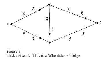
Processes executed to perform a task can often be represented in a task network, as in Fig. 1. Vertex o is the start of the task (typically, stimulus presentation). Each arc represents a process. Associated with each arc is a real number (or random variable), the duration of the process. The processes leaving a vertex all begin when a release condition is met by the processes entering the vertex. A process leaving an AND gate vertex begins execution when all the processes entering the vertex are completed. A process leaving an OR gate vertex begins execution as soon as any process entering the vertex is completed. Vertex r is the end of the task (typically, response execution). The processes are partially ordered by their precedence relation, and so can be represented in a directed acyclic graph. Because mental processes are unobservable, the cognitive psychologist faces an inverse problem, namely, to infer the task network and the durations of the processes from response times measured under various conditions.
Academic Writing, Editing, Proofreading, And Problem Solving Services
Get 10% OFF with 24START discount code
1. Representation Of Processes
The bar chart (or Gannt chart) in Fig. 2 illustrates a model of the psychological refractory period, adapted from Davis (1957) and used recently by Pashler (1998). Two stimuli, o1 and o2 , are presented, requiring responses r1 and r2 , respectively. For stimulus o1 , perceptual processing is denoted a1 , central processing is denoted b1 , and motor preparation is denoted c . Processes for stimulus o are denoted analogously. The interval between the onsets of the stimuli, the stimulus onset asynchrony, is denoted SOA. When process durations are fixed numbers, the length of the bar representing a process indicates its duration. The arrow from the end of b to the beginning of b indicates that b must be completed before b can start, in accordance with Welford’s (1952) single-channel theory.
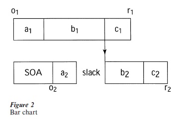
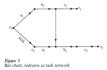
Process durations are easily apprehended from the bar chart, but precedence relations between the processes are not. The bar chart in Fig. 2 can be converted readily to a task network, as in Fig. 3. Precedence relations are seen more easily in the task network, at the cost of losing a visual representation of the process durations.
One use of a task network in scheduling theory is to calculate the time required to complete the task, that is, the response time, from known durations of directed paths through the network. A directed path from vertex u to vertex z is formed by starting at u, going along an arc leaving u to another vertex , and so on, ending at vertex z. There is no directed path from the starting vertex of a process to itself, that is, no directed path is a cycle. Hence a task network is a directed acyclic network. The duration of a path is the sum of the durations of all the arcs on it. If the vertices are AND gates, the network is called a PERT network, and the longest path from o to r is called the critical path. The time to complete the task is the duration of the critical path. If the vertices are OR gates, the time to complete the task is the duration of the shortest path from o to r.
2. Constructing The Network
The key idea for constructing the network is selective influence, pioneered by Sternberg (1969) in his additive factor method. Suppose one experimental factor (say, degrading stimulus quality) prolongs one of the processes, leaving the others unchanged. Suppose another experimental factor (say, increasing response complexity) prolongs another process, leaving the others unchanged. Suppose the processes required for the task are executed one after the other, in series. Then the increase in response time produced by prolonging both processes will be the sum of the increases produced by prolonging them individually.
When process durations are stochastically dependent, factors selectively influencing processes can have unexpected consequences (Townsend and Thomas 1994). The complications arise when a factor prolongs a process p, and the duration of process p is correlated with the duration of a process q; then the duration of process q is changed when the level of the factor is changed. See Dzhafarov (1999) for a general interpretation of selective influence under these circumstances.
2.1 Prolonging A Single Process
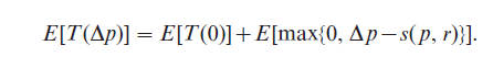
Suppose, for a moment, the process durations are real numbers. When a process p is prolonged by an amount ∆p, the response time need not increase by ∆p. To see this, suppose (until noted otherwise) all vertices are AND gates. In Fig. 1, process x can be prolonged by up to 2 units without increasing the response time. The longest time by which a process p may be prolonged without delaying the response is called the total slack for p, denoted s( p, r). The first s( p, r) units of the prolongation are used to overcome the total slack for p, and the remainder increases the response time. Let T(0) denote the response time when no processes are prolonged and let T(∆p) denote the response time when process p is prolonged by ∆p. Then T(∆p) =T(0) + max 0, ∆p – s( p, r) . Suppose now the process durations and the prolongation of p are random variables. For expected values,
2.2 Prolonging Two Processes
When each of two factors influences selectively a different process, the effects depend on how the two influenced processes are related. (The importance of process arrangements has been advocated continuously by Townsend.) Relations between processes are determined by directed paths. If there is a directed path from the head of a process p to the tail of a process q, then p must be completed before q can start, and p precedes q. Processes p and q are called sequential if either p precedes q or q precedes p. If processes p and q are not sequential, they are concurrent. Concurrent processes p and q can be executed in any order. That is, p and q may be executed simultaneously, or p may be completed before q starts, or q may be completed before p starts.
Assume (a) no process precedes itself (irreflexivity), and (b) if a process p precedes a process q, and q precedes a process t, then p precedes t (transitivity). In other words, precedence is a partial order.
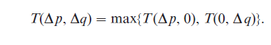
For simplicity, again consider process durations and prolongations as fixed numbers. Let the response time when p is prolonged by ∆p and q by ∆q be denoted T(∆p, ∆q); the notation is analogous for other conditions. Suppose p and q are concurrent processes. The response time when both p and q are prolonged is the larger of the response time when p is prolonged and the response time when q is prolonged, that is,
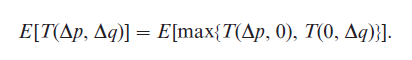
Generally, the times are random variables with expected values,
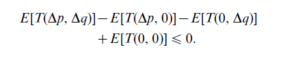
A quantity sensitive to the relation between two prolonged processes is the interaction contrast. For concurrent processes p and q, this quantity is negative or zero, i.e.,
Suppose p and q are sequential processes. When p and q are both prolonged the response time is a complicated function of their respective prolongations, ∆ p and ∆q. Fortunately, when the prolongations are long enough to overcome the relevant slacks, the interaction contrast can be shown to take the following simple form:
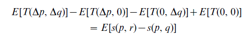
where s(p, q) is the slack from p to q, that is, the longest time by which p can be prolonged without delaying the start of process q.
Ordinarily, the total slack for p is greater than or equal to the slack from p to q, and consequently the interaction contrast for sequential processes is zero or positive. The one exception is processes on opposite sides of a Wheatstone bridge; see x and y in Fig. 1. For such processes, the interaction contrast is zero or negative. In Fig. 1, s(x, r) = 2 ≤ s(x, y) = 4 (considering process durations as fixed numbers), and the interaction contrast is negative. Processes on opposite sides of a Wheatstone bridge can mimic concurrent processes, because both arrangements of processes lead to negative interaction contrasts. The main difference is that for the Wheatstone bridge, when prolongations are long, the value of the interaction contrast does not change as the prolongations become still longer. This is not true for the interaction contrast corresponding to concurrent processes.
When vertices are OR gates, the main difference is a reversal of signs (Schweickert and Wang 1993, Townsend and Nozawa 1995). For concurrent processes, the interaction contrast is positive or zero. For sequential processes not on opposite sides of a Wheatstone bridge, the interaction contrast is negative or zero. For sequential processes on opposite sides of a Wheatstone bridge, the interaction contrast is positive or zero.
2.3 Constructing The Partial Order
Because concurrent and sequential processes behave differently, one can determine which pairs of processes are concurrent and which are sequential. This information is sufficient for constructing a directed acyclic graph. One begins with a comparability graph in which each process is represented by a vertex, and two vertices are joined by an undirected edge if and only if the corresponding processes are sequential. All possible directed acyclic graphs compatible with the comparability graph can then be constructed with the transitive orientation algorithm (Golumbic 1980).
2.4 Estimating Process Durations
If process duration distributions are exponential or general gamma, a reasonable assumption, then the response time can be derived from an order-of-processing (OP) diagram (Fisher and Goldstein 1983). Figure 4 gives the OP diagram for a PERT network in which processes a and b are concurrent and both are followed by process c. Each vertex in the OP diagram is a state, in which certain processes are under way (upper list) and certain others are completed (lower list). The task begins with a and b both under way. In the following states, either a is completed first or b is completed first. Following either of these states, process c is under way. In the final state, process c is completed, and the task is finished.
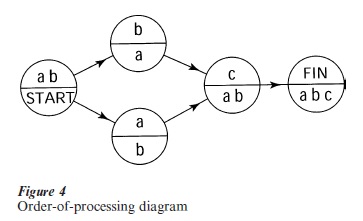
Suppose processes have independent exponential distributions, with the mean of process a denoted 1/λa, and so on. The expected value of the response time can be read off the OP diagram. The first state is completed as soon as the faster of processes a and b is completed. The expected value of the minimum of two independent exponentially distributed processes is itself exponentially distributed, with mean equal to the sum of the means, so the expected value of the duration of the first state is 1/(λa + λb). The probability a is the first process to finish is λa /(λa + λb). Because b is exponentially distributed, the expected value of the time remaining for b to complete given that a has already completed is 1/λb. After repeated application of these rules, the expected value of the response time is the sum over all states of the expected duration of each state multiplied by the probability of reaching that state. For Fig. 4,
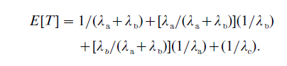
To finish, one can use a nonlinear parameter estimation program to estimate the unknown rates, given observations from enough conditions.
2.5 A Generalization
OP diagrams can represent more general arrangements of processes than those in directed acyclic networks. Consider Fig. 2: if b1 and b2 were sequential, but either could be executed first, the situation cannot be represented by a single directed acyclic network, but can be represented by one OP diagram.
Bibliography:
- Davis R 1957 The human operator as a single channel information system. Quarterly Journal of Experimental Psychology 9: 119–29
- Dzhafarov E N 1999 Conditionally selective dependence of random variables on external factors. Journal of Mathematical Psychology 43: 123–57
- Fisher D L, Goldstein W M 1983 Stochastic PERT networks as models of cognition: Derivation of the mean, variance, and distribution of reaction time using order-of-processing (OP) diagrams. Journal of Mathematical Psychology 27: 121–51
- Golumbic M 1980 Algorithmic Graph Theory and Perfect Graphs. Academic Press, New York
- Pashler H 1998 The Psychology of Attention. MIT Press, Cambridge, MA
- Pinedo M 1995 Scheduling: Theory, Algorithms, and Systems. Prentice Hall, Englewood Cliffs, NJ
- Schweickert R 1978 A critical path generalization of the additive factor method: Analysis of a Stroop task. Journal of Mathematical Psychology 18: 105–39
- Schweickert R, Wang Z 1993 Effects on response time of factors selectively influencing processes in acyclic task networks with OR gates. British Journal of Mathematical and Statistical Psychology 46: 1–30
- Sternberg S 1969 The discovery of processing stages: Extensions of Donders’ method. In: Koster W G (ed.) Attention and Performance II. North-Holland, Amsterdam, pp. 276–315
- Townsend J T, Nozawa G 1995 Spatio-temporal properties of elementary perception: An investigation of parallel, serial, and coactive theories. Journal of Mathematical Psychology 39: 321–59
- Townsend J T, Thomas R D 1994 Stochastic dependencies in parallel and serial models: Effects on systems factorial interactions. Journal of Mathematical Psychology 38: 1–34
- Welford A T 1952 The ‘psychological refractory period’ and the timing of high-speed performance.’ A review and a theory. British Journal of Experimental Psychology 11: 193–210
ORDER HIGH QUALITY CUSTOM PAPER

Always on-time

Plagiarism-Free

100% Confidentiality