Biological Models of Neural Networks Research Paper

1. Modeling The Computational Properties Of Neurons

Although the idea that the brain is the seat of the mind and controller of behavior is many centuries old, research into the computational properties of interconnected neurons was largely absent until the 1940s. McCulloch and Pitts (1943) initiated the field of neural network research by investigating networks of interconnected neurons, with each neuron treated as a simple binary logic computing element. In this model, the axon of a neuron carries the cell’s binary output signal. This axon forms a set of synaptic connections to the dendrites, or inputs, of other neurons. The axonal signal corresponds roughly to the voltage level, or membrane potential, of the neuron. The total input to a neuron is the sum of its synaptic inputs, and if this sum exceeds a certain threshold, the McCulloch–Pitts neuron produces an output of 1. Otherwise the cell’s output is 0. This binary conception of a neuron’s output was based on observations of ‘all or nothing’ spikes, or action potentials, in the membrane potentials of biological neurons.

The McCulloch–Pitts model of the neuron was formulated when our physiological understanding of neurons was rather limited. Although simple binary neurons are still used in some neural network models, many later models treat a neuron’s output as a continuous, rather than binary, function of the cell’s inputs. This change was motivated by neurophysiological observations that the frequency of neuron spiking, rather than the presence or absence of an individual spike, is the more relevant quantity for measuring the strength of signaling between neurons. Perhaps the most widely used formulation of a neuron’s output in current neural networks is the following equation:

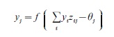
where y_j is the output (spiking rate) of a neuron labeled j, z_ij is the strength of the connection (synapse) from neuron i to neuron j, θ_j is the firing threshold for neuron j, and the output function f (x) is typically an increasing function of x, with f (x) = 0 for x < 0. In words, if a neuron’s total input (Σ_iy_iz_ij) is below the firing threshold, then the neuron’s output is zero, and if the input exceeds the firing threshold, then the output is a positive value related to the difference between the total input and the threshold. Different models use different forms of f (x), with common choices including threshold linear and sigmoidal out- put functions.

A significantly more sophisticated account of neuron dynamics was formulated by Hodgkin and Huxley (1952), who won the Nobel prize for their experimental and modeling work elucidating the relationship between the ionic currents flowing in and out of a neuron and the membrane potential of the neuron. The behavior of networks of Hodgkin– Huxley-like neurons, or shunting neural networks, has been studied in some detail (e.g., Grossberg 1980), and these networks have formed the basis of a number of models of biological nervous systems.

The models described above are point models of a neuron in that they treat the electrical properties of the neuron as uniform across the neuron’s membrane; in other words, they treat neurons as if they did not have a spatial extent. However, the membrane potential of a real neuron varies as a function of position on the membrane. For example, the membrane potential at a distal dendrite of a neuron can differ substantially from the membrane potential at the cell body or along the axon. Sophisticated compartmental models of neurons, which treat the neuron as a collection of interconnected electrical subcircuits (compartments), have been developed in recent years. Each subcircuit in a compartmental model corresponds to a different portion of a real neuron, such as a single dendrite, and large-scale computer simulations are used to simulate the membrane potential of a single neuron. Although compartmental models provide a more accurate description of single neuron dynamics than the point models used in most neural networks, the complexity of this type of model has prevented its use in networks containing more than a handful of neurons. (See Arbib 1995 for more information on single neuron models and neuron simulators.)

2. Learning In Neural Networks

The connections between cells in an artificial neural network correspond to synapses in the nervous system. In the earliest neural network models, the strengths of these connections, which determine how much the presynaptic cells can influence the activity of the postsynaptic cells, were kept constant. However, much of the utility of neural networks comes from the fact that they are capable of modifying their computational properties by changing the strengths of synapses between cells, thus allowing the network to adapt to environmental conditions (for biological neural networks) or to the demands of a particular engineering application (for artificial neural networks). A major challenge for computational neuroscientists has been to develop useful algorithms for changing the weights in a neural network in order to improve its performance based on a set of training samples.

Training a neural network typically consists of the presentation of a set of input patterns alone, or the presentation of input/output pattern pairs, to the network. During the presentation of each pattern or input/output pair, the weights of the synapses in the network are modified according to an equation that is often referred to as a learning law. In a supervised learning network, training consists of repeated presentation to the network of input output pairs that represent the desired behavior of the network. The difference between the network’s output and the training output represents the performance error and is used to determine how the weights will be modified. In a self-organizing network, the weights are changed based on a set of input patterns alone, and the network typically learns to represent certain aspects of the statistical distribution of the training inputs. For example, a self-organizing network trained with an input data set that includes three natural clusters of data points might learn to identify the data points as members of three distinct categories.

A variety of learning laws have been developed for both supervised and self-organizing neural networks. Most of these learning laws fall into one of two classes. The origins of the first class, associative or Hebbian learning laws, can be traced to a simple conjecture penned by the cognitive psychologist Donald Hebb (1949): ‘when an axon of cell A is near enough to excite a cell B and repeatedly or persistently takes part in firing it, some growth process or metabolic change takes place in one or both cells such that A’s efficiency, as one of the cells firing B, is increased.’ With this statement, Hebb gave birth to the concept of Hebbian learning, in which the strength of a synapse is increased if both the preand postsynaptic cells are active at the same time. Remarkably, Hebb’s conjecture, which was made before the development of experimental techniques for collecting neurophysiological data concerning synaptic changes, has proven to capture one of the most commonly observed aspects of synaptic change in biological nervous systems, and variations of the Hebbian learning law are used in many current neural network models. It should be noted, however, that these learning laws are considerably simplified approximations of the complex and varied properties of real synapses.

In a neural network using Hebbian learning, a synapse’s strength depends only on the pre-and postsynaptic cell activations, rather than on a measure of the network’s performance error. Hebbian learning laws are thus well-suited for self-organizing neural networks.

A second common class of neural network learning laws, error minimization learning laws, are commonly employed in supervised learning situations where an error signal can be computed by comparing the network’s output to a desired output. Whereas Hebbian learning laws arose from psychological and neurophysiological analyses, error minimization learning laws arose from mathematical analyses aimed at minimizing the network’s performance error, usually through a technique known as gradient descent. The network’s performance error can be represented as a surface in the space of the synaptic weights. Valleys on this error surface correspond to synaptic weight choices that lead to low error values. Ideally, one would choose the synaptic weights that correspond to the global minimum of the error surface. However, the entire error surface cannot be ‘seen’ by the network during a training trial; only the local topography of the error surface is known. Gradient descent learning laws change the synaptic weights so as to move down the steepest part of the local error gradient.

One of the first gradient descent learning laws was developed by Widrow and Hoff (1960) for a simple one-layer neural network, the ADALINE model, which has found considerable success in technological applications such as adaptive noise suppression in computer modems. However, one-layer networks have limited computational capabilities. Gradient descent learning has since been generalized to networks with three or more layers of neurons, as in the commonly employed back-propagation learning algorithm first derived by Paul Werbos in his 1974 Harvard Ph.D. dissertation and later independently rediscovered and popularized by Rumelhart et al. (1986).

3. Common Neural Network Architectures

The cells in a neural network can be connected to each other in a number of different ways. A feed-forward network is one in which the output of a cell does not affect the cell’s input in any way. Probably the most common artificial neural network architecture is the three-layer feed-forward network, first described by Rosenblatt (1958). In this architecture, an input pattern is represented by cells in the first layer. These cells project through modifiable synapses to the second layer, which is often referred to as the hidden layer since it is not directly connected to the input or output of the network. The hidden layer cells in turn project through modifiable synapses to the output layer. The back-propagation learning algorithm is a common choice for supervised learning in three-layer feed-forward networks.

Recurrent or feedback networks can exhibit much more complex behavior than feed-forward networks, including sustained oscillations or chaotic cycles of cell activities over time. In their most general form, the cell outputs of one layer in a recurrent network not only project to cells in the next layer, but they can also project to cells in the same layer or previous layers. Variants of the back-propagation algorithm have been developed for training multilayer recurrent networks.

One important and heavily studied recurrent network architecture is the self-organizing map, which was first formulated to account for neurophysiological observations concerning cell properties in primary visual cortex (von der Malsburg 1973). The basic principle of a self-organizing map is as follows. Cells in the input layer, sometimes referred to as a subcortical layer, project in a feed-forward fashion to the cells in the second, or cortical, layer, through pathways that have modifiable synapses. Cells in the cortical layer are recurrently interconnected, and they compete with each other through inhibitory connections so that only a small number of the cortical layer cells are active at the same time. These ‘competition winners’ are typically the cells that have the most total input projecting to them from the subcortical layer, or the cells that lie near cells with a large amount of input. The connections between the subcortical cells and the active cortical cells are then modified via an associative learning law so that these cells are even more likely to become active the next time the same input pattern is applied at the subcortical layer. The net effect over many training samples is that cells that are near to each other in the cortical layer respond to similar input patterns (a property referred to as topographic organization), and more cortical cells respond to input patterns that are frequently applied to the network during training than to rarely encountered input patterns. Although originally formulated as recurrent networks in which the cells in the cortical layer project to each other in a recurrent fashion, simplified feed-forward versions of the self-organizing map architecture that approximate stable behavior of the recurrent system have been developed and thoroughly studied (e.g., Kohonen 1984).

A related neural network architecture that has also been used to explain a number of neurophysiological observations is the adaptive resonance theory (ART) architecture (Grossberg 1980). In this network, an additional set of recurrent connections project from the cortical layer back down to the subcortical layer. The top-down projections emanating from a cortical cell embody the subcortical pattern that the network has learned to expect when that cortical cell is activated. These learned expectations can be used to correct coding errors before learning has taken place in the bottom-up pathways, thereby providing a more stable cortical representation. In addition to their use in biological modeling, neural network systems based on the ART model have been applied to a number of pattern recognition problem domains (Carpenter and Grossberg 1991).

4. Specialized Neural Models Of Biological Systems

The neural networks described so far are ‘generalpurpose’ models in that the same architecture is used to attack a variety of biological modeling or engineering problems. In addition to these models, many specialized models of particular neural circuits have been proposed. Among the earliest were models of cerebellum function, proposed by researchers such as Marr and Albus beginning in the late 1960s. The cerebellum has a very regular and well-characterized anatomical structure, and cerebellar physiology has been heavily studied in recent decades. Different cells and synapses in the cerebellum have different properties, and neural models of the cerebellum typically incorporate these differences. Relatively primitive invertebrate neural circuits, such as heartbeat oscillators, have also been the focus of numerous biologically specialized neural network models, as have vertebrate circuits such as the superior colliculus, hippocampus, basal ganglia, and various regions of cortex.

Another type of specialized biological model approximates the function of entire behavioral systems involving large-scale networks of the human brain. Individual cells in these models often correspond to relatively large brain regions, rather than to single neurons or distinct populations of neurons. These models often combine aspects of different neural network architectures or learning laws. The DIVA model of speech production (Guenther 1995), for example, combines several aspects of earlier neural network models into an architecture that learns to control movements of a computer-simulated vocal tract. The model has been shown to provide a unified account for a wide range of experimental observations concerning human speech that were previously studied independently. Other models of this type address various aspects of human cognition, movement control, vision, audition, language, and memory.

5. Pattern Recognition Applications

Neural networks are capable of learning complicated nonlinear relationships from sets of training examples. This property makes them well suited to pattern recognition problems involving the detection of complicated trends in high-dimensional datasets. One such problem domain is the detection of medical abnormalities from physiological measures. Neural networks have been applied to problems such as the detection of cardiac abnormalities from electrocardiograms and breast cancer from mammograms, and some neural network diagnostic systems have proven capable of exceeding the diagnostic abilities of expert physicians. Supervised learning networks have been applied to a number of other pattern recognition problems, including visual object recognition, speech recognition, handwritten character recognition, stock market trend detection, and scent detection (e.g., Carpenter and Grossberg 1991). For further reading on neural networks and their biological bases, see Anderson et al. (1988), Arbib (1995), and Kandel et al. (2000).

Bibliography:

1. Anderson J A, Pellionisz A, Rosenfeld E (eds.) 1988 Neuro-computing. MIT Press, Cambridge, MA
2. Arbib M A (ed.) 1995 The Handbook of Brain Theory and Neural Networks. MIT Press, Cambridge, MA
3. Carpenter G A, Grossberg S (eds.) 1991 Pattern Recognition by Self-Organizing Neural Networks. MIT Press, Cambridge, MA
4. Grossberg S 1980 How does a brain build a cognitive code? Psychological Review 87: 1–51
5. Guenther F H 1995 Speech sound acquisition, coarticulation, and rate effects in a neural network model of speech production. Psychological Review 102: 594–621
6. Hebb D O 1949 The Organization of Behavior: a Neuropsychological Theory. Wiley, New York
7. Hodgkin A L, Huxley A F 1952 A quantitative description of membrane current and its application to conduction and excitation in nerve. Journal of Physiology (Lond.) 117: 500–44
8. Kandel E R, Schwartz J H, Jessell T M (eds.) 2000 Principles of Neural Science, 4th edn. McGraw-Hill, New York
9. Kohonen T 1984 Self-organization and Associative Memory. Springer-Verlag, New York
10. Malsburg C von der 1973 Self-organization of orientation sensitive cells in the striata cortex. Kybernetic 14: 85–100
11. McCulloch W S, Pitts W 1943 A logical calculus of the ideas immanent in nervous activity. Bulletin of Mathematics and Biophysics 5: 115–33
12. Rosenblatt F 1958 The perceptron: A probabilistic model for information storage and organization in the brain. Psychological Review 65: 386–408
13. Rumelhart D E, McClelland J L, PDP Research Group 1986 Parallel Distributed Processing: Explorations in the Microstructure of Cognition. MIT Press, Cambridge, MA
14. Widrow B, Hoff M E (eds.) 1960 Institute of Radio Engineers Western Electric Show and Convention, Institute of Radio Engineers, New York. Reprinted in Anderson J A, Pellionisz A, Rosenfeld E (eds.) 1988 Neuro-computing. MIT Press, Cambridge, MA