Theory Of Stable Populations Reseach Paper

Subject to age-specific mortality and fertility rates which remain unchanged over time a population will eventually develop a stable age distribution which depends on those mortality and fertility rates but is independent of the initial age distribution of the population. This result, due to Sharpe and Lotka (1911) caused renewed interest in stable populations among demographers. Although demographers usually think of a stable population as one with an age distribution which is unchanging, such a definition is restrictive, because populations can also exhibit stability in respect of other characteristics as well as age and in more general situations.

1. The Population Model Of Sharpe And Lotka

Sharpe and Lotka considered the male population alone and assumed that the growth of the female population would be such as to justify assumptions of constant age-specific fertility and mortality for the males. Subsequent writers have usually applied the model to the female component of the population because of its shorter reproductive age span and the fact that the number of females in the reproductive age range plays a more significant role in determining the number of births than the number of males (Pollard 1973).

Applied to the female population, the model assumes F(x, t)dx females in the age range (x, x + dx) at time t and B(t)dt female births between times t and t + dt. Then, if the average number of daughters born per female aged exactly x in time element dt is λ(x)dt and the probability that a female survives from age u to age u + v is _vp_u, the following relationship is immediately apparent:

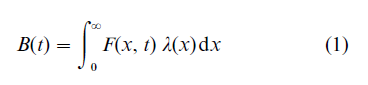
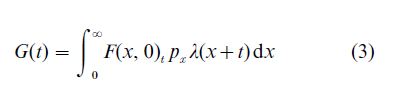
Noting that those alive and aged x at time t, enumerated in F(x, t)dx, must either have been born at time t – x (x < t) or else have been aged x – t at time 0 (x > t), Eqn. (1) may be rewritten as

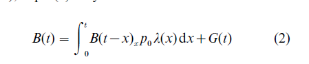
with

The solution to the integral equation (2) reveals that for large values of t, under quite general assumptions

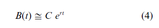
where the constant r (the intrinsic growth rate of the population) is the unique real solution to the integral equation

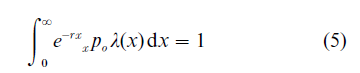
and the constant C depends on the initial age distribution of the population as well as the age-specific mortality and fertility rates (Keyfitz 1968, Pollard 1973).

Since the females aged between x and x dx at time t are the survivors of those born x years earlier between times t – x and t – x + dx, it follows from Eqn. (4) that

The first factor in the right-hand side of Eqn. (6) indicates that the population grows exponentially asymptotically at rate r, while the second reveals that the age distribution is asymptotically independent of t. In other words, a stable age distribution is reached.

2. The Discrete Time Model Of Bernardelli, Leslie, And Lewis

Whilst the continuous time model of Sharpe and Lotka is elegant and predicts a stable population asymptotically under conditions of constant age specific mortality and fertility, the discrete time formulation of Bernardelli (1941), Lewis (1942) and Leslie (1945), which makes similar assumptions, is more readily adapted to analyze stability in more complicated situations.

The number of females aged x last birthday at time t is represented by n_x,t. There is no migration, and no one can live beyond age k last birthday. The average number of daughters born to a female while she is aged x last birthday, those daughters surviving to be enumerated as being aged zero at the next point of time, is F_x, and the proportion of females aged x last birthday surviving to be aged x + 1 last birthday a year later is P_x. Under these assumptions, the following matrix recurrence equation must apply to the numbers of females in successive years:

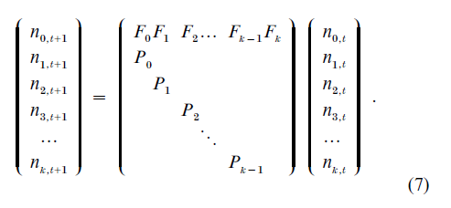
This equation may be written more concisely as

so that

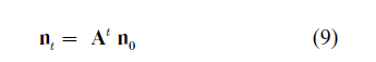
Under fairly general conditions, matrix A is positive regular, in which case it has a dominant eigenvalue α which is positive, of multiplicity one, and greater in absolute size than any other eigenvalue. It follows from Eqn. (9) therefore that for large t,

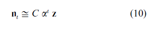
where C is a constant which depends on the initial age distribution of the population, and z is the column eigenvector corresponding to the eigenvalue α. If Π_s is written instead of the product P₀P₁…P_S, the elements of z are Π₀α⁻⁰, Π₁α⁻¹,…, Π_kα^−k. It follows, therefore that the number of females aged x last birth- day at time t is

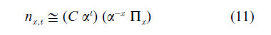
This is the discrete analogue of the Sharpe and Lotka formula, Eqn. (6). The second factor defines the asymptotic stable age distribution; the first shows the exponential growth of the population (Keyfitz 1968, Pollard 1973).

3. Stability With Migration

The most appropriate model for a population subject to significant migration must depend on the pattern that migration takes. In the case of a country accepting a constant number of immigrants each year with a constant age pattern, for example, the discrete time recurrence of Eqn. (8) needs to be modified as follows:

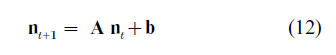
where b is a constant vector of immigrants. Under this model, immigrants are assumed to adopt immediately the mortality and fertility patterns of their new homeland. Repeated application of Eqn. (12) for t = 0, 1, 2, … reveals that, provided the dominant eigenvalue of A is not equal to one,

If the rate of natural increase of the population is less than zero, α will be less than one, and for very large t

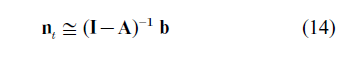
The population will become stationary with its age structure determined by the ages of the immigrants (vector b), as well as the mortality and fertility of the host country (matrix A). Where the fertility of the host country is greater than replacement level, α will be greater than one, and the following asymptotic formula follows from Eqn. (13) for very large t:

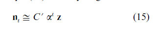
In this case, the population grows asymptotically with the same exponential growth rate as it did in the discrete nonimmigration case of Sect. 2. The asymptotic stable age distribution (vector z) is also the same. The constant C`, however, is different, depending on the initial age structure, the vector of immigrants b, and the mortality and fertility of the population.

In the pathological case where the levels of mortality and fertility in the population correspond exactly to replacement, α is equal to one, and a different algebraic approach is necessary to the solution of Eqn. (12), which yields, for very large t, the following asymptotic result:

The population grows linearly asymptotically and the asymptotic age distribution is the same as in the previous case. The constant C“ depends on the immigration vector, as well as the fertility and mortality rates of the population.

For a population experiencing net emigration with a proportion β_x of females aged x departing each year, the matrix model of Sect. 2 can be utilized with each of the P_x in matrix A replaced by P_x – β_x. The mathematical theory can then be applied in the same manner as before, and an asymptotic stable population emerges. The dominant eigenvalue and eigenvector will of course be different from those in Sect. 2. Depending on whether the dominant eigenvalue of the modified matrix A is less than, equal to, or greater than one, the population will ultimately decline, become stationary or grow in size.

The above models are only two of a very wide range of possible migration models appropriate in different circumstances. They demonstrate how the discrete time model of Sect. 2 may be readily modified to take account of migration and the fact that population stability will usually emerge in the presence of migration when the migration parameters, mortality, and fertility remain unchanged over time.

4. Generalizations

The discrete time models of the earlier sections are readily adapted to study populations partitioned according to other characteristics as well as age. Multiregional demography is the best known example (Rogers 1966, 1975). Females of a population are characterized by age and geographical region in an extended column vector n_t of dimension m_k, where k is the maximum age last birthday attainable and m is the number of regions in the country. As well as surviving and reproducing in the manner of Sect. 2 with rates that may differ from region to region, females can move from one region to another with transition rates which depend on the regions involved and may also depend on age. The matrix recurrence equation is again Eqn. (8), but with n_t of dimension m_k and A of dimension m_k × m_k. Conditions for a unique dominant eigenvector are readily determined, and asymptotic stability for the population by age and geographic region is predicted.

Another partition characteristic sometimes proposed is the parity of woman. Females at time t are enumerated in a vector n_t with elements {n_x,y,t } which record the numbers aged x last birthday who already have y children. The only possible transitions for a female aged x and parity y remaining within the system are to age x + 1 and parity y or to age x + 1 and parity y + 1 (ignoring the small possibility of multiple births). Where there is a change in parity, a new female will be introduced into the population aged 0 last birthday and parity 0 if the mother’s change in parity corresponds to a female birth. Recurrence matrix A contains these transition rates. The fundamental recurrence equation is again Eqn. (8). For all realistic populations, the enlarged matrix A will have a unique dominant eigenvector, and the population enumerated by age and parity will approach stability (Keyfitz 1968).

The discrete-time models of Sects. 2 and 3 have also been applied to workforce planning (Bartholomew 1973, Pollard 1967), membership of learned societies (where Fellows are elected on merit and there is a danger of the society becoming a rapidly aging institution), and membership of other groups including pension schemes (Sherris and Pollard 1980). A learned society, for example, might have a policy of electing five new Fellows each year. The membership of the society at time t can be summarized by a vector n_t with elements n_x,t representing the numbers at the various ages at that time. The number of new members (five) and their age distribution can be summarized in a vector b. The transition rates in the recurrence matrix are simply the proportions {P_x } surviving from age x last birthday to age x + 1 last birthday a year later, for all relevant ages. Assuming that the ages are listed in their natural increasing order, the transition matrix A is particularly simple in this case: all its elements are zero, except those immediately below the main diagonal which comprise the survival proportions {P_x} . With n_t, b, and A defined in this manner, the recurrence equation for the society is Eqn. (12). All the eigenvalues of A are zero, and for t greater than the number of ages involved, A^t= O. The society will approach a stationary state given by Eqn. (14).

All such linear models with realistic assumptions concerning transition between states, entry and reproduction can be shown to predict stable populations asymptotically.

5. Applications

No observed population experiences constant levels of mortality and fertility. Nevertheless the concept of a stable population finds frequent application. Keyfitz’s elegant formula for the effect of population momentum assumes that the population is stable immediately prior to fertility falling to replacement level. Yet the formula works remarkably well for observed populations which are not stable. Stable population theory may be helpful in deducing results in respect of populations with unreliable and/or limited demographic data. Equation (4), for example, can be used to infer an approximate value for the crude birth rate of a population where contraception is not widely practiced, using only a reliable census of the population and a more or less appropriate life table (Bourgeois-Pichat 1957). Many of the applications of model life tables rely on stable population theory.

6. Limitations

The discrete time model of Bernardelli, Leslie, and Lewis, like the continuous (female) formulation of Sharpe and Lotka, assumes that the development of the male component of the population is such as to justify the assumption of unchanging female agespecific mortality and fertility. Linear models which include the male component of the population alongside the females have also been proposed, and mathematical analysis analogous to that presented in Sect. 2 predicts a stable age–gender composition for the whole population. Nonlinear models have also been proposed to accommodate the ‘two-sex problem.’ Many of these nonlinear models would also seem to predict populations which are asymptotically stable under conditions of unchanging rates of mortality, fertility and nuptiality.

For many developing countries, for which stable population theory had been an extremely helpful tool, mortality began to decline in the second half of the twentieth century, but fertility remained essentially unchanged from previous levels. To accommodate the improvements in mortality, the concept of a quasistable population was introduced: one with improving mortality but constant fertility (Coale 1963).

Bibliography:

1. Bartholomew D J 1973 Stochastic Models for Social Processes, 2nd edn. Wiley, New York
2. Bernardelli H 1941 Population waves. Journal of Burma Re- search Society 31: 1–18
3. Bourgeois-Pichat J 1957 Utilisation de la notion de population stable pour mesurer la mortalite et la fecondite des populations des pays sous-developpes Bulletin de l’Institut International de Statistique (actes de la 30e Session)
4. Coale A J 1963 Estimation of various demographic measures through the quasi-stable age distribution. Emerging Techniques in Population Research: Proceedings of the 1962 Annual Conference of the Milbank Memorial Fund
5. Keyfitz N 1968 Introduction to the Mathematics of Population. Addison-Wesley, Reading, MA
6. King G 1902 Life Contingencies, 2nd edn. Charles & Edward Layton, London
7. Leslie P H 1945 On the use of matrices in certain population mathematics. Biometrika 33: 183–212
8. Lewis E G 1942 On the generation and growth of a population. Sankhya 6: 93–6
9. Pollard J H 1967 Hierarchical population models with Poisson recruitment. Journal of Applied Probability 4: 209–13
10. Pollard J H 1973 Mathematical Models for the Growth of Human Populations. Cambridge University Press, Cambridge, UK
11. Rogers A 1966 The multiregional matrix growth operator and the stable interregional age structure. Demography 3: 537–44
12. Rogers A 1975 Introduction to Multiregional Mathematical Demography. Wiley, New York
13. Sharpe F R, Lotka A J 1911 A problem in age-distribution. Philosophical Magazine, Ser. 6 21: 435–8
14. Sherris M, Pollard J H 1980 Application of matrix methods to pension funds. Scandinavian Actuarial Journal 77–95