Theory of Nonstable Populations Research Paper

Suppose the number of children born in period t is B_t, and the child survival rate is l, then N_t = l . B_t−1. The above two equations can be combined in the following reduced form: B_t = h(B_t−1), where h(B_t) = g(f (l . Bt₋₁)) . l . B_t−1. The above expression is a recursive equation of B_t, from which the dynamic pattern can be analyzed, and the possible existence of cyclicity can be studied. Here the Malthusian model is interpreted as a model of density dependency, where the density is characterized by the birth size of the previous period. It turns out that the Malthusian model described above may not converge to a ‘dismal’ steady state, as Malthus suggested. Mathematically, the B_t series may converge, diverge, or be cyclic, and the volatility of the birth series B_t crucially hinges on the feedback elasticity of h (.) with respect to B_t−1. When this elasticity is sufficiently large, the B_t series can easily have cycles. This is the classical case of nonstable population. Modern versions of nonstable population will be discussed below, after we introduce the general population structure.

2. The General Population Structure

Let N_t = (N_t,1, …, N_t,n) be an n-type population vector at period t, where N_{t, i}, i = 1,…, n indicates the size of type-i population at period t. The type here may refer to any criterion that is used to classify the population, such as age, sex, and occupation. A general formulation of population dynamics can be written as follows:

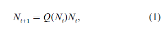
where Q(N_t) is the transition matrix. The simplest case is when Q(N_t) = Q, a time-independent matrix. In this situation, the above equation reduces to a time- invariant Markov chain: N_t+1 =QN_t. It is a well-known implication of the Frobenius–Perron theorem that if Q is positively regular, meaning that there is flexible cross-period mobility across types, then the population vector N_t will converge to a steady state, in which all elements of the N_t vector grow at the same exponential rate, thereby the population composition is also time-invariant. It has been shown by Chu (1998) that, for most population models with time- independent Q, this positive regularity condition is likely to be satisfied, therefore any nonstable behavior of the population would appear only when Q(N_t) is not a constant matrix, or equivalently when the relationship between N_t+1 and N_t in Eqn. (1) has some nonlinearity. Below we shall introduce several special cases of the generic setting in Eqn. (1), and discuss their empirical relevance. The reader can see that each model corresponds to a special interpretation of the generic setting in Eqn. (1).

3. Easterlin Cycles

For demographers, the most familiar version of the dynamic models in Eqn. (1) is the Lotka–Leslie agespecific models, where the type criterion is age. Let N_{t, I} be the number of population aged i at period t, Bt−i be the birth size at period t – i, and l_i be the probability that a person can survive to age i, then the following relationship must hold: N_{t, i} = B_t−i l_i. The transformed dynamics in terms of B_t is the well-known Lotka’s equation:

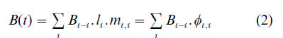
where m_{t, i} is the average number of births per surviving member aged i at period t, and φ_{t, i} = l_i . m_{t, i} is the net maternity function. Evidently, the Malthusian model presented in the previous section is a special case of Eqn. (2a) with two age types. As we mentioned, when the fertility function m_{t, i} is independent of t, then the process of B_t follows a time-invariant Markov chain, and the usual convergence result applies. But if m(t,i) is time dependent, then cycles or more volatile behavior may appear. One typical case of such time dependency is when the age-specific fertility rates are functions of previous birth sizes: m_{t, i} = m_i(B_t), where B_t = (B_t−1, B_t−2,…).

Suppose the birth series corresponding to Eqn. (2a) has a steady state. Taking a Taylor expansion around this steady state, Lee (1974) showed that the volatility of the birth series characterized by Eqn. (2a) hinges upon the elasticities of the net maternity function with respect to B_t. When previous birth sizes are larger, usually the density pressure is larger. Intuitively, larger feedback elasticities imply that present reproduction would be more sensitive to previous birth shocks, hence the birth series would be more volatile. Easterlin (1961) argued that the baby-boom baby-bust cycles observed in the United States are typical examples of a feedback cycle.

How large the feedback elasticities are is an empirical question. In order to estimate such elasticities, two models have been proposed: the first is to assume that φ_{t, i} is only a function of the cohort size aged i: φ_t,i = φ_i (B_t−i), and the second is to assume that φ_{t, i} is a function of the weighted average of birth sizes of different ages: φ_{t, i} = φ_i( ∑_j w_j . B_t−j ). The former is referred to as the cohort model, and the latter as the period model. However, empirical evidence has so far failed to back up either of these two models in producing persistent birth cycles that fit all characteristics (such as amplitude and period). Moreover, even if there does exist a cyclic solution to Eqn. (2a), the information concerning feedback elasticity is not sufficient for us to tell whether the cyclical solution in question is stable. Related analysis is rather technical, and the reader is referred to Tuljapurkar (1987) for details.

4. Predator–Prey Cycles

The predator–prey model describes a two-type population structure, where the types are prey and predator, respectively, referred to as type-1 and type-2. The simplest formulation of the predator–prey model is characterized by the following difference equations:

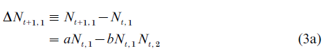
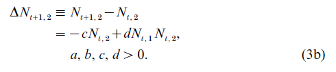
Equation (3) is obviously a special case of Eqn. (1). The prey are considered the only food resource available to the predator. Thus, if N_t,1 =0, the predator population decreases exponentially at the rate c. With the nonexistence of predators, the prey population grows exponentially at the rate a.

In the steady state of Eqn. (3), ∆N_t,1 = ∆N_t,2 = 0, there is only one nontrivial solution: (N₁*, N₂*) (c/d, a/b). Let the Jacobian matrix of Eqn. (3) around the nontrivial solution be denoted J. It turns out that the determinant of J is

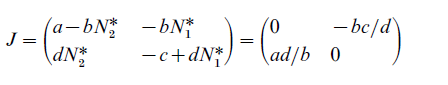
|J|= ac > 0 and the trace of J is zero.

Thus, we know that the eigenvalues of J are purely imaginary, meaning that besides the equilibrium point (c/d, a/b) itself, the solution trajectories of Eqn. (3) are cyclic and nonstable. But it was also pointed out that when the predator–prey model embodies the concerns of diminishing or increasing returns, then the solution becomes locally stable or divergent.

5. Dynastic Cycles

Based on stylized facts found in Chinese history, Chu and Lee (1994) proposed an occupation-specific population model, in which the population is separated into three occupations: bandits, peasants, and soldiers. Peasants grow crops and pay taxes, soldiers (rulers) collect taxes and hunt for bandits, and bandits rob food and clash with peasants and soldiers. It is assumed that soldiers are drafted by the government, and all other civilians can choose to become peasants or bandits. Their occupation choice is made depending on which occupation is expected to generate a higher utility. When the bandit soldier ratio is relatively high, it is likely that the incumbent power regime will be overthrown by the bandit group, and the dynasty switches. It turns out that this pattern of population dynamics characterizes the dynamic evolution of dynasties in Chinese history, and the cycles were called dynastic cycles by historians.

In terms of demography, the occupation switches mentioned above are merely changes in population composition. But there is a unique feature associated with the above-mentioned occupation switching, which we shall explain below. For most animals, it is believed that when density pressure occurs, the environment becomes less favorable, and the reproduction rate of animals is reduced. One might expect that rational human decisions may be able to weaken the outside density pressure through institutional and rational regulation. But the scenario of dynastic cycles seems to be a counterexample. As noted by historians, clashes between soldiers and rebellious peasants in human history were often initiated by famine or density pressure. The higher the bandit ratio, the less likely a peasant can safely keep a good proportion of his crop, and hence the greater attraction for the peasant to join the bandit group and seize other people’s crops. Thus, human beings’ occupational choice between peasants and bandits has a ‘demonstration effect,’ which tends to magnify the originally weak density pressure and ‘destablize’ the dynamics of the population compositional structure.

The cyclical pattern of population composition mentioned above is not the only case we find in human history. Some researchers have considered a neoclassical economic growth model, and focused on the two economic classes in the economy: the laborers and the capitalists. Let u_t be the income share attributed to labor, and t be the employment rate of labor. Under some reasonable assumptions, Goodwin (1967) has shown that the dynamics of u_t and t mimic that of Eqn. (3). Thus, the conclusion that the capitalists’ economy appears to be ‘permanently oscillating’ was reached. But just as the original predator–prey model is sensitive to variations in institutional specifications, Goodwin’s model after some minor modification also generates qualitatively different results. Definite evidence of the nonstability of human population has yet to be found.

Bibliography:

1. Cyrus Chu C Y 1998 Population Dynamics: A New Economic Approach. Oxford University Press, New York
2. Cyrus Chu C Y, Lee R D 1994 Famine, revolt and the dynastic cycle: Population dynamics in historic China. Journal of Population Economics 7: 351–78
3. Easterlin R A 1961 The American baby boom in historical perspective. American Economic Review 51: 860–911
4. Goodwin R M 1967 A growth cycle. In: Feinstein C H (ed.) Socialism, Capitalism and Economic Growth. Cambridge University Press, Cambridge, UK
5. Lee R 1974 The formal dynamics of controlled population and the echo, the boom and the bust. Demography 11: 563–85
6. Tuljapurkar S 1987 Cycles in nonlinear age-structured models i: Renewal dynamics. Theoretical Population Biology 32: 26–41