Multistate Transition Models In Demography Research Paper

1. Increment-Decrement Tables

During the 1960s and the 1970s, demographic work on multistate life tables produced a generalization of classical mathematical techniques used in demography for more than 300 years. These new models can be viewed as superimposing a set of two or more life statuses on the single dimension of the classical life table, which only has a live-to-dead transition. For example, they can incorporate several forms of decrement from an initial state, such as mortality by cause of death in multiple-decrement tables. They can also chain together a series of multiple-decrement tables without permitting reentries into a state previously occupied, such as transitions to rising educational levels in hierarchical tables. They finally lead to more general nonhierarchical increment-decrement tables, which accommodate reentrants into states and differentiate interstate moves by both origin and destination (Land and Rogers 1982), as in multiregional migration models.

These models describe the dynamics of populations where individuals in a given state are assumed to be homogeneous: the probability to move from one state to another is the same for all individuals in the same state. Population heterogeneity can be accounted for to some extent by increasing the number of possible states. However, the introduction of a growing number of subpopulations in order to ensure homogeneity in each state quickly leads to group sizes so small as to rule out all analysis. What is more, one can never be sure of having taken into account every factor of heterogeneity.

1.1 A Marko Chain Formulation

Mathematics allows us to develop tools to describe transitions between the various observed states. One considers an individual life course as the result of a stochastic process occurring in the given state space. The time dimension may represent biological age or duration since some initial event, for example, time since entry into the labor force. This process is said to satisfy the Markov property if its present state is all that counts in predicting its future: what other states were occupied previously by the individual has no effect on the coming move. The future is independent of the past except through the present. The process is not always stationary, as transition probabilities may depend on time. This leads to time-continuous Markov chain models with a finite state space.

Consider a single sample path, and let I_i (t) = 1 if it is in state i at time t, with I_i(t) = 0 otherwise. One defines the transition intensity from state i to state j at time t as

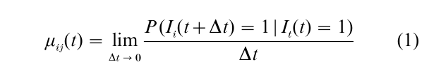
For increment-decrement tables only aggregate data on flows between states are used; one does not use individual trajectories in the calculations. In some cases transition intensities may be specified as given functions that are known except for the value of parameters that must be estimated from the observed data. In other cases one uses approximations such as piecewise constant intensities provided time intervals are available over which the intensities can be taken as constant. Once these transition intensities are estimated, one may find the corresponding transition probabilities for every suitable time period, for example, the probability that an individual in state i at time t₁ will be in state j at time t₂. It is also useful to estimate expected sojourn times in each state and many other summaries of behavior. Finally, these analyses may be completed using regression models with aggregate characteristics for each state.

The availability of aggregate or contextual data may invite the analyst to examine the effect that characteristics of the groups studied have on group behavior. The aggregate or contextual characteristics are interpreted as a set of constraints that each subpopulation imposes on its members (or corresponding opportunities) and which influences their behavior. For example, such an analysis may perhaps reveal a positive association between the rate of unemployment in a region and its out-migration rate. But there is a real danger of inferring from such an observation that individuals of this population who are unemployed have a higher probability of out-migrating from a region, whereas all that is identified by the model is that a high rate of unemployment is accompanied by a high rate of out-migration, whether the individuals involved are economically active, unemployed, or inactive. This type of mistaken inference from group-level associations to individual behavior is known as the ecological fallacy. Committing this fallacy is avoided in event-history analysis, which is discussed later.

1.2 More Complex Models

The Markov chain assumption is restrictive and constitutes a rough approximation for many demographic processes. For example, in migration analysis one needs to account for duration dependence in the propensity to move. There are also preferred patterns of moves between regions; for instance, return moves back to a region of origin are preferred to moves to other regions. Such features can be taken into account using more complex models.

The first way to analyze non-Markovian processes is to expand the state space so that the process in the new space is Markovian. Such an extension, however, again leads to an increase of the amount of data necessary to estimate the large number of transition intensities beyond what is possible with the usual data sets. A second possibility lies in the use of a semi-Markov process. In such a model the probability of moving at a given time can bear any arbitrary relation to the duration of stay (Ginsberg 1971). Nevertheless, any extension leaves out some property of the studied process and even more complex models are needed. For example, in the case of migration a semi-Markov process is unable to take into account the higher probability of return moves unless one introduces information about previously occupied states.

2. Multistate Event-History Models

Increment-decrement tables are computed primarily from aggregate data. It will normally be preferable to use individual-level data instead. This approach allows us to examine how events that occur to an individual can influence their future life course and how personal characteristics can give individuals behavior patterns that are different from those of other individuals. Event history models have been developed to deal with such information, mainly during the 1980s.

2.1 Interaction Between Events

Again a mathematical formulation helps us analyze the issues involved (Andersen et al. 1993). Let P_i(t) be the number of individuals observed in state i just before time t and let M_ij(t) be the number of observed transitions from state i to state j during the time interval [0, t]. Then the vector M = {M_ij, i = j} is a multivariate counting process where M_ij has intensity process µ_ij(t)P_i(t). Here µ_ij(t) is the corresponding transition intensity.

With these tools it is possible to follow each individual and to study interactions between various processes. Consider the links between family formation and urban migration in France, for example. In this country, the metropolitan areas are centered on Paris, Lyons, and Marseilles, and using data for the years 1925 to 1950 Courgeau (1989) followed women who lived in these areas or outside them on their 14th birthday. For these women, childbearing intensities for birth orders higher than one turned out to depend strongly on whether they had migrated or not. For women from outside the metropolitan areas, migration to such an area reduced their fertility by one third. Conversely, migration to a nonmetropolitan area brought about a sharp rise in fertility for women from the cities. After migration, cumulative childbearing intensities were 1.4 to 2 times higher than for those who remained in the metropolitan area where they started out. Migration to a metropolitan area attracted women whose fertility before migration was already similar to that prevailing in the urban area, and they displayed selective behavior. Migration to a less urbanized area attracted women whose fertility before migration was similar to that of other women in the urban area, and the women showed adaptive behavior.

Conversely, the birth of successive children also influenced women’s mobility; there is reciprocal dependence. The intensity of moving to a metropolitan area was reduced after each successive birth, but that of moving in the opposite direction was increased slightly by these births.

This analysis illustrates the complex dependencies that can be observed between various dimensions of behavior, in this case childbearing and migration. We can speak of local dependence when there is a one-sided influence of one process on the other without reciprocity (Schweder 1970), and of total independence if at any time each event occurs independently of the other, though this rarely occurs in practice. For even more complex dependencies, see Courgeau and Lelievre (1992).

It is possible to enlarge the ambit of the analysis to cover situations with even more states. For example, one can consider studying fertility occurring in various types of partnership (marriage or cohabitation), or interactions between fertility and changes of residence.

2.2 Population Heterogeneity

Suppose that each individual carries a collection of possibly time-dependent characteristics which may change at distinct points in time due to outside influences and also on the influence of the individual’s own previous life history. The effect of these characteristics on the events of interest is investigated via a time-dependent regression model, which may be a generalization of the Cox (1972) model and may allow us to model the hazard or intensity using fixed and time-dependent covariates.

Consider an individual k with a vector of possibly time-varying characteristics Z^k(t) at time t. We write his hazard rate (or intensity) for a transition from state i to state j as

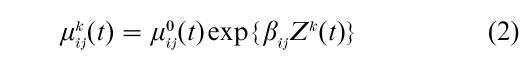
where the baseline hazard (intensity) µ_ij⁰(t) is the same for all individuals and each β_ij is a vector of parameters that measure the impact of the covariates. Individual- level covariates may be binary (being married or not), polytomous (being (a) economically active and employed, (b) unemployed, or (c) economically inactive), a feature that can be treated as continuous (such as income), or even more diverse. An analysis based on such a model can reveal whether individuals who are unemployed have a higher probability of migrating out of a region than employed individuals, for instance, a result which cannot be shown with aggregate data.

Courgeau (1989) used such a model to reconsider the interaction between the birth of the third child and mobility, taking into account individual characteristics. Some of these characteristics turned out to be affected by the migration process in France. Being the daughter of someone engaged in agriculture had an effect on such a birth irrespective of whether the woman lived in a metropolitan area or not, for instance. Before migration this would delay the birth, but after a move the effect disappeared. Other aspects of behavior were not affected by this migration. For example, if a woman had a large number of siblings, she would be more likely to have a third child irrespective of whether she came from a rural or an urban background. Once these different effects were taken into account, the migration to metropolitan areas continued to induce a marked reduction in the chance of giving birth to a third child, whereas migration to less urbanized areas always raised fertility.

However, as one can never be sure to have collected information on all aspects that might explain a given behavior, unobserved heterogeneity may be an issue. When it is independent of the characteristics observed, it reduces the absolute value of the estimates of regression parameters β_ij that represent the effect of observed characteristics, but it does not change their sign (Bretagnole and Huber-Carol 1988). When the observed characteristics turn out to have a significant effect, one can then conclude that this will not be modified by independent unobserved heterogeneity; but when no significant effects are found, a real effect can be disguised by unobserved heterogeneity.

There are various ways of accounting for unobserved heterogeneity, but a common procedure is to posit a set of individual-level scalar random effects V^k_ij that are added in the exponent of the intensity function, as in

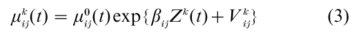
These random variables are then supposed to represent selectively and/or heterogeneity in the population by picking up effects of covariates that are not included in the intensity-regression analysis.

Even when these powerful tools are used, care is needed, given that one frequently specifies behavior as influenced only by the characteristics of the individual. The danger here is of committing the atomistic fallacy if no attention is paid to the context in which human behavior occurs. In point of fact, this context often does have an influence, in which case it is fallacious to consider individuals in isolation from the constraints and opportunities imposed by the society and milieu in which they live. Contextual variables may be aggregates of individual level characteristics (such as the percent married in the individual’s region of residence) or general contextual characteristics (such as the number of hospital beds in the same region or its political color). More complex analytical procedures can also be employed (such as the average income or the correlation between income and matrimonial status).

Formally, contextual variables appear in the formulas above simply as factors Z^k(t) whose values are common to all individuals k who live in the same context.

3. Contextual And Multilevel Analysis

The need to introduce the influence of contextual characteristics has given rise to the idea of working simultaneously on different levels of aggregation with the aim of explaining a behavior which is treated as individual rather than aggregated as in increment-decrement tables. This removes the risk of committing the ecological fallacy, since a characteristic on the aggregate or contextual level is only used to measure an influence that may be different from its equivalent at the individual level. It is introduced not as a substitute but as a feature of the subpopulation, a feature that influences the behavior of an individual who belongs to it. And the atomistic fallacy is also eliminated once the context in which the individual lives is specified correctly in the analysis.

The main limitation of contextual analysis is that the behaviors of individuals in the same context are treated as independent. Such an assumption is usually not true, as the behavior of an individual in a group often depends on other individuals in the same group. Think of members of a family or household, or citizens of a town. One may need to take into consideration the observed social structure of a group and the interactions that exist between its members as well as changes in such interactions over time (Lelievre et al. 1998). Ignoring within-group dependence may lead to estimated variances of contextual effects that are biased downward, making confidence intervals too narrow. To handle this problem one extends the contextual model, following a development that took place during the late 1980s and in the 1990s. Here is a quick sketch of the main principles of such an extension.

Suppose that individuals are organized into groups and that individual k in group h has transition intensities of the form

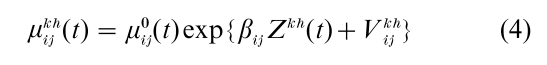
Modern software like aML (see Lillard and Panis 2000) can handle analyses of such models. There is much interest currently in how one can identify sensible distributions for the heterogeneity variables {V^ij_kh} and {W_ij^h} (‘mixing distributions’) (see Horowitz 1999).

Multilevel analysis can be extended to more than two levels. The simplest and more widely used structure is hierarchical: each level is formed by grouping together of all units of the previous level: pupils are grouped in classes, which in turn are in schools, which are perhaps divided between the state and private sector, and so on. The relationship between the levels can be more complicated: individuals can be grouped in towns of ascending size order, but distinguished also between administrative, industrial, and tourist centers, for example. In this case there is a cross-classification that includes towns being classified by size and by function, say. It is of course, possible to have relationships that combine hierarchical and cross-classifications. For example, individuals may be classified by type of residential neighborhood and by type of place of work (cross-classification), which are themselves placed in a hierarchical classification of parishes and regions.

It is not necessary to study a single process alone, as when moves between different states of one kind are considered independently of other changes occurring simultaneously in other life domains. Dynamic multilevel event-history analysis can be used to study several interrelated processes at the same time. For instance, the study of fertility in the various regions of a country can be carried out, in principle, simultaneously with a study of migration between the regions, and this may be useful since some women change residence between the regions during their reproductive period.

4. Conclusion

Improvements in multistate analysis such as that sketched here are the subject of current research. One can expect much future development in the epistemological bases, methods of measurement, and procedures of analysis of a dynamic theory of human behavior along these lines.

Bibliography:

1. Andersen P, Borgan O, Gill R, Keiding N 1993 Statistical Models Based on Counting Processes. Springer-Verlag, New York
2. Bretagnole J, Huber-Carol C 1988 Effects of omitting covariates in Cox’s model for survival data. Scandinavian Journal of Statistics 15: 125–38
3. Courgeau D 1989 Family formation and urbanization. Population: An English Selection 1: 123–46
4. Courgeau D 1995 Migration theories and behavioural models. International Journal of Population Geography 1: 19–27
5. Courgeau D, Baccaıni B 1998 Multilevel analysis in social science. Population: An English Selection 10: 39–71
6. Courgeau D, Lelievre E 1992 Event History Analysis in Demography. Clarendon, Oxford, UK
7. Cox D 1972 Regression models and life tables (with discussion). Journal of the Royal Statistical Society B34: 187–220
8. Ginsberg R 1971 Semi-Markov processes and mobility. Journal of Mathematical Sociology 1: 233–62
9. Goldstein H 1995 Multilevel Statistical Models. Arnold, London
10. Hoem J, Funck Jensen U 1982 Multistate life table methodology: A probabilistic critique. In: Land K, Rogers A (eds.) Multidimensional Mathematical Demography. Academic Press, New York
11. Horowitz J L 1999 Semiparametric estimation of a proportional hazard model with unobserved heterogeneity. Econometrica 76(5): 1001–28
12. Keilman N 1993 Emerging issues in demographic methodology. In: Blum J, Rallu L (eds.) European Population, II— Demographic Dynamics. John Libbey INED, Paris
13. Land K, Rogers A (eds.) 1982 Multidimensional Mathematical Demography. Academic Press, New York
14. Lelievre E, Bonvalet C, Bry X 1998 Event history analysis of groups. The findings of an on-going research project. Population: An English Selection 10: 11–37
15. Lillard L A, Panis C W A 2000 aML Multilevel Multiprocess Statistical Software, Release 1.0. Econ-Ware, Los Angeles
16. Schweder T 1970 Composable Markov processes. Journal of Applied Probability 7: 400–10