Single-Case Experimental Designs Research Paper

In practice, most research involves elements of both traditions, but the extensive study of individual cases has led to some of the most important discoveries in the behavioral sciences and therefore has a special place in the history of scientific discovery. Single-case or single-subject design (also known as ‘N of one’) research is often employed when the researcher has limited access to a particular population and can therefore study only one or a few subjects. This method is also appropriate when one wishes to make an intensive study of a phenomenon in order to examine the conditions that maximize the strength of an effect. In clinical settings one is frequently interested in describing which variables affect a particular individual rather than in trying to infer what might be important from studying groups of subjects and assuming that the average effect for a group is the same as that observed in a particular subject. In the current era of increased accountability in clinical settings, single-case design can be used to demonstrate treatment effects for a particular clinical case (Hayes et al. 1999 for a discussion of the changing research climate in applied settings).

2. Characteristics Of Single-Case Design

Single-case designs study intensively the process of change by taking many measures on the same individual subject over a period of time. The degree of control in single-case design experiments can often lead to the identification of important principles of change or lead to a precise understanding of clinically relevant variables in a specific clinical context. One of the most commonly used approaches in single-case design research is the interrupted time-series. A time-series consists of many repeated measures of the same variable(s) on one subject, while measuring or characterizing those elements of the experimental context that are presumed to explain any observed change in behavior. An by examining characteristics of the data before and after the experimental manipulation to look for evidence that the independent variable alters the dependent variable because of the interruption.

3. Specific Types Of Single-Case Designs

Single-case designs frequently make use of a graphical representation of the data. Repeated measures on the dependent variable take place over time, so the abscissa (X-axis) on any graph represents some sort of across time scale. The dependent measure or behavior presumably being altered by the treatment is plotted on the ordinate (Y-axis). There are many variations of single-case designs that are well described (e.g., Franklin et al. 1997, Hersen and Barlow 1976, Kazdin 1982), but the following three approaches provide an overview of the general methodology.

3.1 The A-B-A Design

The classic design that is illustrative of this approach is called the A-B-A design (Hersen and Barlow 1976, pp. 167–97) where the letters refer to one or another experimental or naturally observed conditions presumed to be associated with the behavior of importance. A hypothetical example is shown in Fig. 1. By convention, A refers to a baseline or control condition and the B indicates a condition where the behavior is expected to change. The B condition can be controlled by the experimenter or alternatively can result from some naturally occurring change in the environment (though only the former are true experiments). The second A in the A-B-A design indicates a return to the original conditions and is the primary means by which one infers that the B condition was the causal variable associated with any observed change from baseline in the target or dependent variable. Without the second A phase, there are several other plausible explanations for changes observed during the B phase besides the experimental manipulation. These include common threats to internal validity such as maturation or intervening historical events coincidental to initiating B.

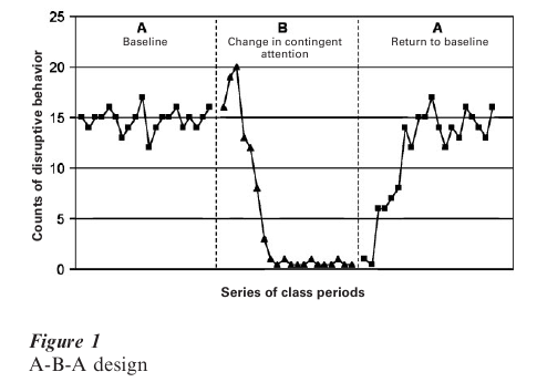
To illustrate the clinical use of such an approach, consider the data points in the first A to indicate repeated observations of a child under baseline conditions. The dependent variable of interest is the number of disruptive behaviors per class period that the child exhibits. A baseline of disruptive behaviors is observed and recorded over several class periods. During the baseline observations, the experimenter hypothesizes that the child’s disruptive behavior is under the control of contingent attention by the teacher. That is, when the child is disruptive, the teacher pays attention (even negative attention) to the child that unintentionally reinforces the behavior, but when the child is sitting still and is task oriented, the teacher does not attend to the child. The experimenter then trains the teacher to ignore the disruptive behavior and contingently attend to the child (e.g., praise or give some token that is redeemable for later privileges) when the child is emitting behavior appropriate to the classroom task. After training the teacher to reinforce differentially appropriate class- room behavior, the teacher is instructed to implement these procedures and the B phase begins.

Observations are made and data are gathered and plotted. A decrease in the number of disruptive behaviors is apparent during the B phase. To be certain that the decrease in disruptive behaviors is not due to some extraneous factor, such as the child being disciplined at home or simply maturing, the original conditions are reinstated. That is, the teacher is instructed to discontinue contingently attending to task-appropriate behavior and return to giving corrective attention when the child is disruptive. This second A phase is a return to the original conditions. The plot indicates that the number of disruptions returns to baseline (i.e., returns to its previous high level). This return to baseline in the second A condition is evidence that the change observed from baseline condition A to the implementation of the intervention during the B phase was under the control of the teacher’s change in contingent attention rather than some other factor. If another factor were responsible for the change, then the re-implementation of the original baseline conditions would not be expected to result in a return to the original high levels of disruptive behavior.

There are many variations of the A-B-A design. One could compare two or more interventions in an A-B- A-C-A design. Each A indicates some baseline condition, the B indicates one type of intervention, and the C indicates a different intervention. By examining differences in the patterns of responding for B and C, one can make treatment comparisons. The notation of BC together, as in A-B-A-C-A-BC-A, indicates that treatments B and C were combined for one phase of the study.

3.2 The Multiple-Baseline Design

An A-B-A or A-B-A-C design assumes that the treatment (B or C) can be reversed during the subsequent A period. Sometimes it is impossible or unethical to re-institute the original baseline conditions (A). In these cases, other designs can be used. One such approach is a multiple-baseline design. In a multiple-baseline design, baseline data are gathered across several environments (or behaviors). Then a treatment is introduced in one environment. Data continue to be gathered in selected other environments. Subsequently the treatment is implemented in each of the other environments, one at a time, and changes in target behavior observed (Poling and Grossett 1986).

In the earlier example, if the child had been exhibiting disruptive behavior in math, spelling, and social studies classes, the same analysis of the problem might be applied. The teachers or the researcher might not be willing to reinstitute the baseline conditions if improvements were noted because of its disruptive effects on the learning of others and because it is not in the best interests of the child. Figure 2 shows how a multiple-baseline design might be implemented and the data presented visually. Baseline data are shown for each of the three classroom environments.

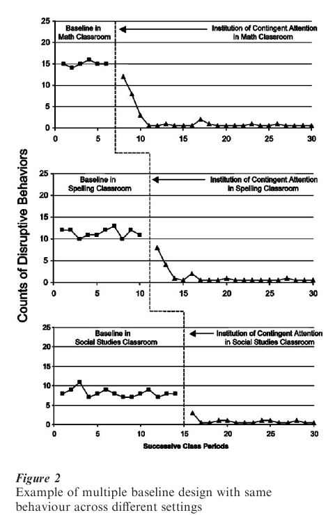
While the initial level of disruptive behavior might be slightly different in each class, it is still high. The top graph in Fig. 2 shows the baseline number of disruptive behaviors in the math class. At the point where the vertical dotted line appears, the intervention is implemented and its effects appear to the right of dotted line. The middle and bottoms graphs show the same disruptive behaviors for the spelling and social studies class. No intervention has yet been implemented and the disruptive behavior remains high and relatively stable in each of these two classrooms. This suggests that the changes seen in the math class were not due to some other cause outside of the school environment or some general policy change within the school, since the baseline conditions and frequency of disruptive behaviors are unchanged in the spelling and social studies classes. After four more weeks of baseline observation, the same shift in attention treatment is implemented in the spelling class, but still not in the social studies class. The amount of disruptive behavior decreases following the treatment implementation in the spelling class, but not the social studies class.

This second change from baseline is a replication of the effect of treatment shown in the first classroom and is further evidence that the independent variable is the cause of the change. There is no change in the social studies class behavior. This observation provides additional evidence that the independent variable rather than some extraneous variable is responsible for the change in the behavior of interest. Finally, the treatment is implemented in the social studies class with a resulting change paralleling those occurring in the other two classes when they were changed. Rather than having to reverse the salutary effects of a successful treatment as one would in an A-B-A reversal design, a multiple baseline design allows for successively extending the effects to new contexts as a means of demonstrating causal control.

Multiple-baseline designs are used frequently in clinical settings because they do not require reversal of beneficial effects to demonstrate causality. Though Fig. 2 demonstrates control of the problem behavior by implementing changes sequentially across multiple settings, one could keep the environment constant and study the effects of a hypothesized controlling variable by targeting several individual behaviors. For example, a clinician could use this design to test whether disruptive behavior in an institutionalized patient could be reduced by sequentially reinforcing more constructive alternatives. A treatment team might target aggressive behavior, autistic speech, and odd motor behavior when the patient is in the day room. After establishing a baseline for each behavior, the team could intervene first on the aggressive behavior while keeping the preexisting contingencies in place for the other two behaviors. After the aggressive behavior has changed (or a predetermined time has elapsed), the autistic speech behavior in the same day room could be targeted, and so on for the odd motor behavior. The logic of the application of a multiple baseline design is the same whether one studies the same behavior across different contexts or different behaviors across the same context. To demonstrate causal control, the behavior should change only when it is the target of a specific change strategy and other behaviors not targeted should remain at their previous baselines.

Interpretation can be difficult in multiple-baseline designs because it is not always easy to find behaviors that are functionally independent. Again, consider the disruptive classroom behavior described earlier. Even if one’s analysis of teacher attention to disruptive behavior is reinforcing, it may be difficult to show change in only the targeted behavior in a specific classroom. The child may learn that alternative behaviors can be reinforced in the other classrooms and the child may alter his or her behavior in ways that alter the teacher reactions, even though the teachers in the other baseline classes did not intend to change their behavior. Nevertheless, this design addresses many ethical and practical concerns about A-B-A (reversal) designs.

3.3 Alternating Treatment Design

The previous designs could be referred to as within-series designs because there are a series of observations within which the conditions are constant, an intervention with another series of observations where the new conditions are constant for the duration of series, and so on. The interpretation of results is based on what appears to be happening within a series of points compared with what is happening within another series. Another variation of the single-case design that is becoming increasingly recognized for its versatility is the alternating treatment design (ATD) (Barlow and Hayes 1979). The ATD can be thought of as a betweenseries design. It is a method of answering a number of important questions such as assessing the impact of two or more different treatment variations in a psychotherapy session. In an ATD, the experimenter rapidly and frequently alternates between two (or more) treatments on a random basis during a series and measures the response to the treatments on the dependent measure. This is referred to as a ‘betweenseries’ because the data are arranged by treatments first and order second rather than by order first, where treatments vary only when series change. There may be no series of one particular type of treatment, although there are many of the same treatments in a row.

To illustrate how an ATD might be applied, consider a situation where a therapist is trying to determine which of two ways of relating to a client produces more useful self-disclosure. One way of relating is to ask open-ended questions and the other is to ask direct questions. The dependent variable is a rating of clinically useful responsiveness from the client. The therapist would have a random order for asking one of the two types of questions. The name of the design does not mean that the questions alternate back and forth between two conditions on each subsequent therapist turn, but randomly change between treatments. One might observe the data in Fig. 3.

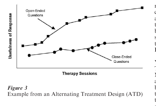
The X-axis is the familiar time variable and the Y-axis the rating of the usefulness of the client response. The treatment conditions are shown in separate lines. Note that points for each condition are plotted according to the order in which they were observed, but that the data from each condition are joined as if they were collected in one continuous series (even though the therapists asked the questions in the order of O-C-O-O-O-C-C-O …). The data in Fig. 3 indicate that both methods of asking questions produce a trend for the usefulness of the information to increase as the session goes on. However, the open-ended format produces an overall higher degree of utility.

4. Analyses

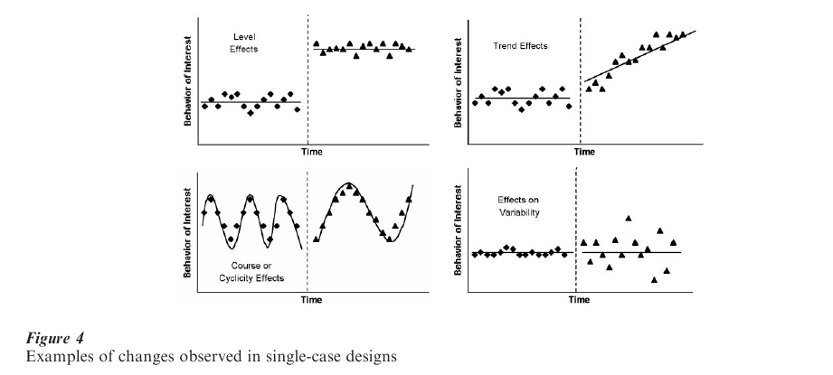
There are four characteristics of a particular series that can be compared with other series. The first is the level of the dependent measure in a series. One way in which multiple series may differ is with respect to the stable level of a variable. The second way in which multiple series may differ is in the trend each series shows. The third characteristic that can be observed is the shape of responses over time. This is also referred to as the course of the series and can include changes in cyclicity. The last characteristic that could vary is the variability of responses over time. Figure 4 shows examples of how these characteristics might show treatment effects. One might observe changes in more than one of these characteristics within and across series.

4.1 Visual Interpretation Of Results

In single-case design research, there has been a long tradition to interpret the data visually once it has been graphed. In part, this preference emerged because those doing carefully controlled single-case research were looking for large effects that should be readily observable without the use of statistical approaches. Figure 4 depicts examples of clear effects. They demonstrate the optimal conditions for inferring a treatment effect, a stable baseline and clearly different responses during the post baseline phase. Suggestions for how to interpret graphical data have been described by Parsonson and Baer (1978).

However, there are many circumstances where patterns of results are not nearly so clear and errors in interpreting results are more common. When there are outlier data points (points which fall unusually far away from the central tendency of other points in the phase), it becomes more difficult to determine reliably if an effect exists by visual inspection alone. If there are carry-over effects from one phase to another that the experimenter may not initially anticipate, results can be difficult to interpret. Carry-over is observed when the effects of one phase do not immediately disappear when the experiment moves into another phase. For example, the actions of a drug may continue long after a subject stops taking the drug, either because the body metabolizes the drug slowly or because some irreversible learning changes occurred as a result of the drug effects. It is also difficult to interpret graphical results when there is a naturally occurring cyclicity to the data. This might occur when circumstances not taken into account by the experimenter lead to systematic changes in behaviors that might be interpreted as treatment effects. A comprehensive discussion of issues of visual analysis of graphical displays is provided by Franklin et al. (1996).

4.2 Traditional Measurement Issues

Any particular observation in a series is influenced by three sources of variability. The experimenter intends to identify systematic variability due to the intervention. However, two other sources of variability in an observation must also be considered. These are variability attributable to measurement error and variability due to extraneous sources, such as how well the subject is feeling at the time of a particular observation. Measurement error refers to how well the score on the measurement procedure used as the dependent measure represents the construct of interest. A detailed discussion of the reliability of measurement entails some complexities that can be seen intuitively if one compares how accurately one could measure two different dependent measures. If the experimenter were measuring the occurrence of head-banging behavior in an institutionalized subject, frequency counts would be relatively easy to note accurately once there was some agreement by raters on what constituted an instance of the target behavior. There would still be some error, but it would be less than if one were trying to measure a dependent measure such as enthusiasm in a classroom. The construct of enthusiasm will be less easily characterized and have more error associated with its measurement and therefore be more likely to have higher variability.

As single-case designs are applied to new domains of dependent measures such as psychotherapy research, researchers are increasingly attentive to traditional psychometric issues, including internal and external validity as well as to reliability. Traditionally, if reliability was considered in early applications of single-case designs, the usual method was to report interrater reliability as the percent agreement between two raters rating the dependent measure (Page and Iwata 1986). Often these measures were dichotomously scored counts of behaviors (e.g., a behavior occurred or did not occur). Simple agreement rates can produce inflated estimates of reliability. More sophisticated measures of reliability are being applied to single-case design research including kappa (Cohen 1960) and variations of intraclass correlation coefficients (Shrout and Fleiss 1979) to name a few.

4.3 Statistical Interpretation Of Results

While the traditional method of analyzing the results of single-case design research has been visual inspection of graphical representation of the data, there is a growing awareness of the utility of statistical verification of assertions of a treatment effect (Kruse and Gottman 1982). Research has shown that relying solely on visual inspection of results (particularly when using response guided experimentation) may result in high Type I error rates (incorrectly concluding that a treatment effects exists when it does not).

However, exactly how to conduct statistical analyses of time-series data appropriately is controversial. If the data points in a particular series were individual observations from separate individuals, then traditional parametric statistics including the analysis of variance, t-tests, or multiple regression could all be used if the appropriate statistical assumptions were met (e.g., normally distributed scores with equal variances). All of these statistical methods are variations of the general linear model. The most significant assumption in the general linear model is that residual errors are normally distributed and independent. A residual score is the difference between a particular score and the score predicted from a regression equation for that particular value of the predictor variable. The simple correlation between a variable and its residual has an expected value of 0. In single-case designs, it can be the case that any particular score for an individual is related to (correlated with) the immediately preceding observation. If scores are correlated with their immediately preceding score (or following score), then they are said to be serially dependent or autocorrelated. Autocorrelation violates a fundamental principle of traditional parametric statistics.

An autocorrelation coefficient is a slightly modified version of the Pearson correlation coefficient (r). Normally r is calculated using pairs of observations (X_i,Y_i) for several subjects. The autocorrelation coefficient (ρ_k) is the correlation between a score or observation and the next observation (Y_i,Y_i+1). When this correlation is calculated between an observation and the next observation, it is called a lag 1 autocorrelation. The range of the autocorrelation coefficient is from -1.0 to +1.0. If the autocorrelation is 0, it indicates that there is no serial dependence in the data and the application of traditional statistical procedures can reasonably proceed. As ρ_k increases, there is increasing serial dependence. As ρ_k becomes negative, it indicates that there is a rapid cyclicity pattern. A lag can be extended out past 1 and interesting patterns of cyclicity may emerge. In economics, a large value of ρ_k at a lag 12 can indicate an annual pattern in the data. In physiological psychology, lags at 12 or 24 may indicate a systematic diurnal or circadian rhythm in the data.

Statistical problems emerge when there is an autocorrelation among the residual scores. As the value of ρ_k increases (i.e., there is a positive autocorrelation) for the residuals, the computed values of many traditional statistics are inflated, and type I errors occur at a higher than expected rate. Conversely, when residuals show a negative autocorrelation, the resulting statistics will be too small producing misleading significance testing in the opposite direction. Suggestions for how to avoid problems of autocorrelation include the use of distribution-free statistics such as randomization or permutation tests. However, if the residuals are auto correlated even these approaches may not give fully accurate probability estimates (Gorman and Allison 1996, p. 172).

There are many proposals for addressing the autocorrelation problem. For identifying patterns of cyclicity, even where cycles are embedded within other cycles, researchers have made use of spectral analysis techniques, including Fourier analysis. These are useful where there may be daily, monthly, and seasonal patterns in data such as one might see in changes in mood over long periods of observation.

The most sophisticated of these approaches is called the autoregressive integrated moving average analysis or ARIMA method (Box and Jenkins 1976). This is a regression approach that tries to model the value of particular observation as a function of the parameters estimating the effects of past observations (φ), moving averages of the influence of residuals on the series (θ), and the removal of systematic trends throughout the entire time series. The computation of ARIMA models is a common feature of most statistical computer programs. Its primary limitation is that it requires many data points, often more than are practical in applied or clinical research settings. Additionally, there may be several ARIMA models that fit any particular data set, making results difficult to interpret. Alternative simplifications of regression-based analyses are being studied to help solve the interpretive problems of using visual inspection alone as a means of identifying treatment effects (Gorman and Allison 1996).

4.4 Generalization Of Findings And Meta-Analysis

Although single-case designs can allow for convincing demonstrations of experimental control in a particular case, it is difficult to know how to generalize from single-case designs to other contexts. Single-case design researchers are often interested in specific effects, in a specific context, for a specific subject. Group designs provide information about average effects, across a defined set of conditions, for an average subject. Inferential problems exist for both approaches. For the single-case design approach, the question is whether results apply to any other set of circumstances. For the group design approach, the question is whether the average result observed for a group applies to a particular individual in the future or even if anyone in the group itself showed an average effect.

In the last two decades of the twentieth century, meta-analysis has become used as a means of aggregating results across large numbers of studies to summarize the current state of knowledge about a particular topic. Most of the statistical work has focused on aggregating across group design studies. More recently, meta-analysts have started to address how to aggregate the results from single-case design studies in order to try to increase the generalizability from this type of research. There are still significant problems in finding adequate ways to reflect changes in slopes (trends) between phases as an effect size statistic, as well as ways to correct for the effects of autocorrelation in meta-analysis just as there are for the primary studies upon which a meta-analysis is based. There is also discussion of how and if single-case and group design results could be combined (Panel on Statistical Issues and Opportunities for Research in the Combination of Information, 1992).

5. Summary

Technical issues aside, the difference between the goal of precision and control typified in single-case design versus the interest in estimates of overall effect sizes that are characteristic of those who favor group designs makes for a lively discussion about the importance of aggregation across studies for the purpose generalization. With analytic methods for single-case design research becoming more sophisticated, use of this research strategy to advance science is likely to expand as researchers search for large effects under well specified conditions.

Bibliography:

1. Barlow D H, Hayes S C 1979 Alternating treatments design: One strategy for comparing the effects of two treatments in a single subject. Journal of Applied Behavior Analysis 12: 199–210
2. Box G E P, Jenkins G M 1976 Time Series Analysis, Forecasting, and Control. Holden-Day, San Francisco
3. Cohen J A 1960 A coefficient of agreement for nominal scales. Educational and Psychological Measurement 20: 37–46
4. Franklin R D, Allison D B, Gorman B S 1997 Design and Analysis of Single-case Research. Lawrence Erlbaum Associates, Marwah NJ
5. Franklin R D, Gorman B S, Beasley T M, Allison D B 1996 Graphical display and visual analysis. In: Franklin R D, Allison D B, Gorman B S (eds.) Design and Analysis of Single-case Research. Lawrence Erlbaum Associates, Marwah NJ, pp. 119–58
6. Gorman B S, Allison D B 1996 Statistical alternatives for single-case designs. In: Franklin R D, Allison D B, Gorman B S (eds.) Design and Analysis of Single-case Research. Lawrence Erlbaum Associates, Marwah NJ, pp. 159–214
7. Hayes S C, Barlow D H, Nelson-Gray R O 1999 The Scientistpractitioner: Research and Accountability in the Age of Managed Care, 2nd edn. Allyn and Bacon, Boston
8. Hersen M, Barlow D H 1976 Single Case Experimental Designs: Strategies for Studying Behavior Change. Pergamon Press, New York
9. Kazdin A E 1982 Single Case Research Designs: Methods for Clinical and Applied Settings. Oxford University Press, New York
10. Kruse J A, Gottman J M 1982 Time series methodology in the study of sexual hormonal and behavioral cycles. Archives of Sexual Behavior 11: 405–15
11. Page T J, Iwata B A 1986 Interobserver agreement: History, theory, and current methods. In: Poling A, Fuqua R W (eds.) Research Methods in Applied Behavior Analysis: Issues and Advances. Plenum, New York, pp. 99–126
12. Panel on Statistical Issues and Opportunities for Research in the Combination of Information 1992 Contemporary Statistics: Statistical Issues and Opportunities for Research. National Academy Press, Washington, DC, Vol. 1
13. Parsonson B S, Baer D M 1978 The analysis and presentation of graphic data. In: Kratochwill T R (ed.) Single-subject Research: Strategies for Evaluating Change. Academic Press, New York, pp. 101–65
14. Poling A, Grossett D 1986 Basic research designs in applied behavior analysis. In: Poling A, Fuqua R W (eds.) Research Methods in Applied Behavior Analysis: Issues and Advances. Plenum, New York
15. Shrout P E, Fleiss J L 1979 Intraclass correlations: Uses in assessing rater reliability. Psychological Bulletin 86: 420–8