View sample cancer research paper on cancer survival. Browse other research paper examples for more inspiration. If you need a thorough research paper written according to all the academic standards, you can always turn to our experienced writers for help. This is how your paper can get an A! Feel free to contact our writing service for professional assistance. We offer high-quality assignments for reasonable rates.
Introduction
It is of considerable interest to know the outcome of treatment for all cancer patients in a population. Clinical trials or studies of hospital records cannot provide this information. Trials include patients who are selected on the basis of strict inclusion and exclusion criteria such as a restricted age range or a lack of serious comorbidity. Trials focus on a pragmatic comparison of efficacy between treatment regimens: They are generally quite small (a few hundred or occasionally a few thousand patients), and in general fewer than 10% of all adult cancer patients are included in trials, even in developed countries. Hospital statistics can only indicate the fate of patients who have been referred to that hospital. The criteria for referral to a given hospital are not usually explicit, and the statistics on outcome are most unlikely to be representative of any population.
Academic Writing, Editing, Proofreading, And Problem Solving Services
Get 10% OFF with 24START discount code
In contrast, the public health interest in cancer survival is in the outcome for all cancer patients. Population-based cancer survival estimates are used to monitor trends in survival over time, as one measure of overall progress in cancer control. They can display breakthroughs in cancer treatment, as happened for childhood cancers in the 1970s and 1980s. They provide a basis for resource estimation for cancer care and a baseline for planning of the clinical trials. They are used to assess inequality in the outcome of cancer between population subgroups defined by age, sex, social class or degree of affluence, and race or ethnic group, or to compare survival between regions within a country or with other countries. Survival estimates provide a crucial measure of the overall efficacy of the entire cancer patient pathway, from the initial health-seeking behavior of a person with symptoms that may be due to cancer, through primary care, referral to secondary care for investigation and diagnosis, and the efficacy and accessibility of available treatment resources. All these uses of cancer survival figures require that the estimates be statistically robust and adequately comparable.
Population-based survival estimates should include the outcome for all cancer patients in a given population. For this reason, the data are usually derived from a population-based cancer registry that collects information on all persons diagnosed with cancer who are normally resident in the region or country covered by that registry. Further reference here to cancer survival will be to population-based estimates, unless otherwise stated.
It is worth considering whether the follow-up of cancer patients, to ascertain their vital status, is in fact required in order to estimate cancer survival, since cancer mortality rates should also reflect survival, and they are routinely available in many countries. Mortality rates cannot be used for this purpose, however. First, mortality reflects both incidence and survival; in other words, the number of deaths from a given cancer will reflect the number of people who are diagnosed with it, as well as their chances of surviving it. In a steady state, therefore, mortality from a very common cancer with good survival could be higher than mortality from an uncommon cancer with poor survival. Second, the deaths from cancer in a given year will arise not just in patients who were diagnosed in that year, but also those diagnosed up to ten or more years earlier, and this backscatter of diagnoses will vary with the lethality of the cancer and with any recent advances in treatment for that cancer. For this reason, mortality trends can rarely offer more than a delayed and blurred reflection of the public health impact of advances in treatment. Third, the accuracy of cancer mortality statistics depends on the accuracy of death certification, and of the coding of the underlying cause of death; both these components of mortality statistics vary with the type of cancer, as well as between countries and over time. For these reasons, mortality statistics are not an adequate surrogate for cancer survival in the context of public health.
Public interest in international comparisons of population-based cancer survival has increased in recent years (Berrino et al., 2003). Such comparisons can be useful for understanding national survival data and for the interpretation of incidence rates. They serve as broad indicators of the quality of patient care. For example, the EUROCARE studies have clearly demonstrated lower survival among cancer patients in several Eastern European countries than in Western European countries, differences that are directly attributable to inferior diagnosis and treatment.
Observed Patient Survival
Survival and the duration of life after diagnosis have been considered to be among the most important indicators of success in the management of cancer patients. In what follows, the analysis of survival is demonstrated in detail. The method is also applicable to the analysis of other clinical outcomes, e.g., relapses or side effects of treatment.
A characteristic problem with follow-up studies is that the patients have different potential follow-up times. A patient diagnosed a long time ago can, potentially, be followed up for much longer than a patient who was diagnosed only recently. It is much more likely that the death of a patient with a long potential follow-up time will be observed than the death of a patient with a short potential follow-up time. Because the times of death are not usually available for all patients, it is not advisable to calculate a mean of the observed survival times, whether of all patients or only of those who have died. Again, because of these differences in potential follow-up time, it is also inappropriate to calculate direct proportions of survivors after certain fixed durations of follow-up time. Those proportions can be obtained by special methods, such as the life table method or the product-limit (Kaplan-Meier) method.
Let us take the colon cancer patients diagnosed in Finland during 1992–2002 as an example. The follow-up time of the patients starts on the date of diagnosis and ends with the date of death, or emigration or 31 December 2003, whichever comes first. Thus, the potential follow-up time for patients diagnosed during 1999–2002 was less than 5 years, whereas it was more than 10 years for patients diagnosed during 1992–93. The actual follow-up was shorter than the potential follow-up for any patient who died or emigrated before 31 December 2003.
Nonlocalized colon cancer was diagnosed in 1230 males aged 60–74 (Table 1). During the first month of follow-up, 53 died from colon cancer and nine from other causes of death. During the second month, 90 died, 79 from colon cancer and 11 from other causes.
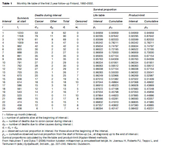
The life table has a row for each interval (month) of follow-up i, including the number of patients alive and under follow-up at the beginning of the interval (li), the number of deaths during the interval (di), and the number of persons who were alive when withdrawn or lost to follow-up at some point during the interval (wi). For months 13–24, the number of withdrawals includes patients diagnosed in 2002 who were still alive on 31 December 2003, when follow-up in the study ceased. Those patients had only been followed up for 1–2 years; their follow-up is said to have been censored (i.e., cut short) after the last possible date on which their death could have been observed.
Loss to follow-up is a good reason for censoring a patient’s follow-up time in the analysis, since the patient is no longer under observation, and a death could not be observed. In Finland, it is rare for cancer patients to move abroad, and because of highly efficient population and death registration systems, it is also rare to lose patients from follow-up. In many other countries, however, withdrawals will also include both patients known to have emigrated and patients who have been lost to follow-up.
The interval-specific observed survival proportion in Table 1, pi, is an estimate of the probability that a patient who is alive at the beginning of interval i will survive until the end of it. This proportion is often incorrectly called a rate (Elandt-Johnson, 1975). The observed survival proportion can be calculated from the formula:

This is simply the complement of the proportion of deaths among those who started the interval, with a correction for censoring, in which we assume that the wi patients who did not die but who were not followed up throughout the entire interval were, on average, followed up until the mid-point of the interval.
The cumulative observed survival proportion up to a given time interval since diagnosis, which is an estimate of the corresponding probability of survival, is obtained by calculation of the product:

This quantity gives an estimate of the probability of surviving i intervals (months) from the start of follow-up. For the 24th month, for example, the observed survival proportion is p24 = 0.98394, while the 24-month (2-year) cumulative observed survival proportion is 24po = 0.40147 (Table 1).
This formula for the survival proportion is based on an assumption that the probability of surviving for those who could not be followed after interval i is the same as the probability of survival for those who were successfully followed up during subsequent intervals. This is called the assumption of independence between dying and censoring.
The assumption may well be valid, but even if follow-up information is complete, problems can arise when the data set includes patients who were diagnosed a long time ago. Obviously, patients diagnosed a long time ago have longer potential follow-up times than patients diagnosed recently, for whom the observed follow-up will thus end more frequently with the patient being censored alive (death has not been observed). Patients whose follow-up times are censored are assumed to have had the same pattern of survival after censoring as patients whom it was possible to follow up for longer, i.e., generally those patients who were diagnosed a longer time ago. Since survival generally improves with time, however, this assumption is not necessarily valid. Under those circumstances, therefore, the cumulative observed survival proportion is likely to be somewhat too low.
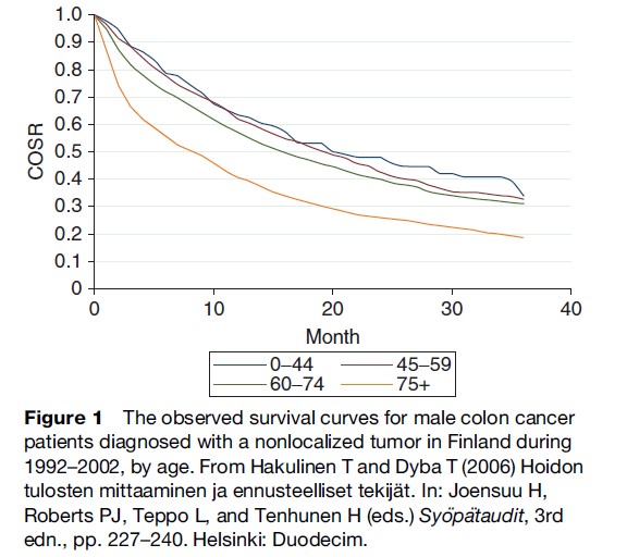
The consecutive estimates of the cumulative observed survival proportion can be joined up to produce observed survival curves (Figure 1). The older the patients, the lower is the cumulative observed survival. The use of straight lines to connect the survival estimates illustrates the idea that deaths within each time interval are evenly spaced in time.
With the product-limit (Kaplan-Meier) method, it is assumed that the times of different events are exactly known. The survival times are then tabulated individually by observed lengths, not by fixed subintervals as in Table 1. In order to apply the product-limit method to the material in Table 1, a decision must be made on how to treat apparently simultaneous deaths and censorings, i.e., those that occur during the same interval. Most computer programs are set to assume that withdrawals (events in the wi column) would happen slightly later than deaths, although there is no particular logical basis for this choice. The survival proportion pi will then be calculated from the formula:
![]()
The number of withdrawals is used only to obtain a new value li+1 = li – di – wi. Otherwise, the calculations are the same as with the usual life-table method outlined above.
Observed survival curves obtained with the productlimit method are step functions, that is, they run horizontally (constant survival proportion) in the intervals between deaths, then drop vertically when deaths occur. In practice, the life-table method and the product-limit method give nearly the same results when the time intervals are short, on the order of 1 month.
The 2-year cumulative observed survival proportion can also be estimated by annual intervals; results are virtually identical. The choice of subintervals for the life-table method depends on the cancer and on the desired degree of detail. The intervals may be unequal, e.g., short intervals at the start of follow-up, when deaths are more frequent, and longer intervals later on, when deaths are less frequent. Intervals should not be longer than 1 year. The assumption of exact event times with the product-limit method requires intervals no longer than 1 month. The life-table method with longer, say, yearly intervals is efficient in summarizing survival information when the data set is large, as is typically the case with population-based cancer registries.
Cause-Specific Survival
Figure 1 The observed survival curves for male colon cancer patients diagnosed with a nonlocalized tumor in Finland during 1992–2002, by age. From Hakulinen T and Dyba T (2006) Hoidon tulosten mittaaminen ja ennusteelliset tekija¨ t. In: Joensuu H, Roberts PJ, Teppo L, and Tenhunen H (eds.) Syo¨pa¨taudit, 3rd edn., pp. 227–240. Helsinki: Duodecim.
We cannot conclude from Figure 1 that colon cancer is more fatal in older patients. The probability of survival for older people is lower in part because of mortality due to other causes of death. If the cause of death of each patient is known, it is possible to calculate cause-specific survival proportions to estimate the probability of survival in the hypothetical situation where colon cancer is the only cause of death. The cause-specific survival proportion in each interval (Table 1) can be obtained as:

Here, deaths from the cancer of interest in the ith interval are counted as events, d1i, while deaths from other causes (d2i) are considered as censorings (compare this formula with that for observed survival in the previous section). Thus the follow-up time has been cut short (censored) by the death of the patient, but the death is not considered as an event of interest for this particular analysis, if it is not a death from the cancer being studied and is therefore not included in the numerator of the estimate of the proportion who have died. In this context, therefore, as with other reasons for censoring the follow-up, deaths from other causes than the cancer of interest are assumed to occur, on average, at the mid-point of the interval.
The cumulative, cause-specific survival proportion is simply the product of the interval-specific proportions, as before:

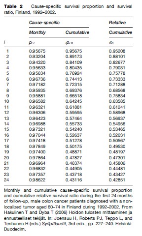
At the end of the 2nd year of follow-up, the cumulative cause-specific survival proportion 24pco ¼ 0.43116 (Table 2) is slightly higher than the observed survival proportion 0.40147 (Table 2).
With the product-limit approach to estimating causespecific survival, the assumption of independence is more difficult to accept than for observed survival, particularly if the patient group is very heterogeneous with respect to age. This is because the risk of death from the cancer and the risk of death from other causes are usually both higher in older patients. This introduces dependence between the risk of death (from the specific cancer) and the risk of censoring (death from another cause). The usual approach to eliminating most of this dependence is to analyze survival by age group. If this is not done, the resulting survival estimate will be too high, because the follow-up of older patients will more often be censored due to death from other causes, and censored patients are assumed to have the same survival experience as those who were not censored, who are on average younger, and in fact have better survival. In other words, censoring for other causes removes from the analysis a group of patients (the elderly) whose actual survival is lower than average, leading to an inflated estimate of overall survival.
The cumulative cause-specific survival proportions may be used to construct cumulative cause-specific survival curves. While the range of the observed 3-year cumulative survival proportions is from 19% (patients aged 75 years or more at diagnosis) to 34% (those aged 0–44 years), the range of the cause-specific survival proportions is 24–34%. Colon cancer is thus more fatal for older patients.
Relative Survival
If the cause of death of the cancer patients is not known, or unreliable, the cause-specific survival can be estimated by using the relative survival ratio, i.e., the ratio of the survival actually observed in the cancer patients and the survival that would be expected in the absence of cancer. Relative survival is thus a ratio of two survival proportions.
The expected survival of the cancer patients is estimated from mortality in the general population, using life tables by sex, age, calendar period, and possibly also other factors such as region, social class or degree of deprivation, and race. This can be done in Finland for the patients in Table 1 by using the general population life tables by sex, age, and time. Thus, if the patients in Table 1 were a sample of the general population in Finland, their expected survival proportion would be pi* = 0.9974 during each month within the 1st year of follow-up and pi* = 0.9972 during each of the following 12 months. The 2-year expected survival proportion would then be 24p0* = 0.93725.
Relative survival in the 1st month of follow-up for the patients in Table 1 is thus r1 = p1/p1* = 0.94959/0.9974 = 0.95208. The ratio in the 2nd month is r2 = p2/p2* = 0.92295/0.9974 = 0.92535. The 2-year cumulative relative survival is 24p0/24p0* = 0.40147/0.93725 = 0.42851 (Table 2).
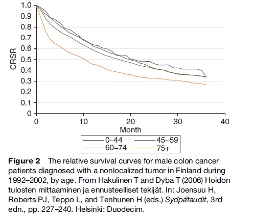
Relative survival can be interpreted as the cause-specific survival, i.e., an estimate of the probability of survival if the patient’s cancer were the only cause of death. Because of the method of calculation, this interpretation is not always strictly possible. Sometimes, particularly when the life table intervals are short and the mortality in the cancer patients is low, the relative survival in a particular time interval may exceed the value of one. This leads to slight upward turns in a survival curve, such as the curve for the youngest age group in Figure 2.
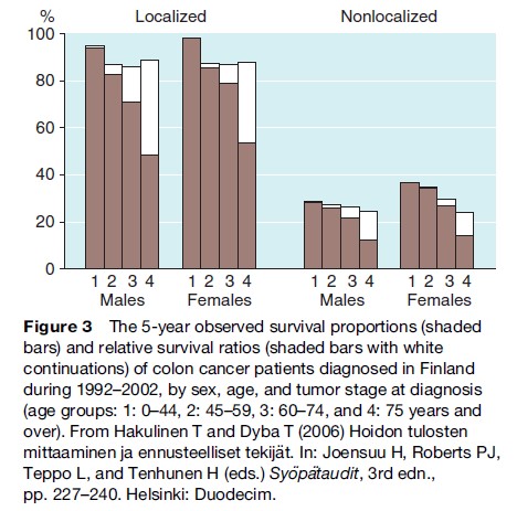
Five-year relative survival for colon cancer is highest in females when the tumor is localized and lowest in males with nonlocalized tumors (Figure 3). Relative survival is lowest for the oldest patients. The variation in relative survival by age is much smaller than for the corresponding observed survival estimates, particularly when the tumor is localized at diagnosis.
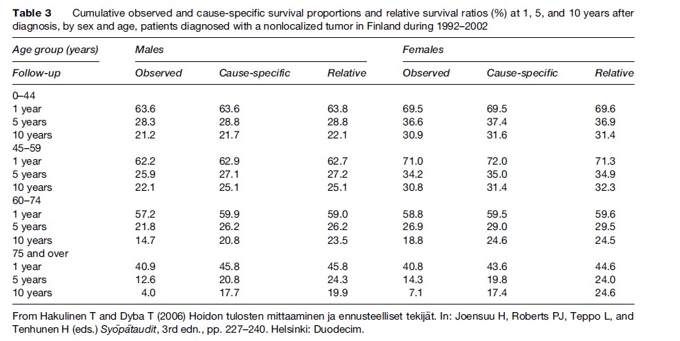
The 5-year relative survival ratios and the cause- specific survival proportions for colon cancer patients are generally similar (Table 3). The differences increase with age and with follow-up time since diagnosis. It is difficult to conclude which estimates of survival are more correct when the differences are large. Knowledge that the patient has cancer may influence the physician’s assessment and certification of the cause of death. On the other hand, cause-specific 15-year survival of those aged 75 years or more at diagnosis may not be of such great interest in practice.
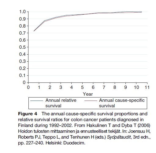
It is important to know when cancer patients are cured. This can be estimated from either the relative survival ratio or the cause-specific survival proportion within successive intervals of time since diagnosis. The estimates should be close to 100% for cured patients. For cause-specific survival, cure implies that patients surviving up to that point would no longer die from their disease. For relative survival, cure would imply that patients surviving up to that point have approximately the same mortality as a comparable group of the general population. On the basis of these quantities, the point of cure for Finnish colon cancer patients occurs around 9 years after diagnosis (Figure 4).
Confidence Intervals And Tests
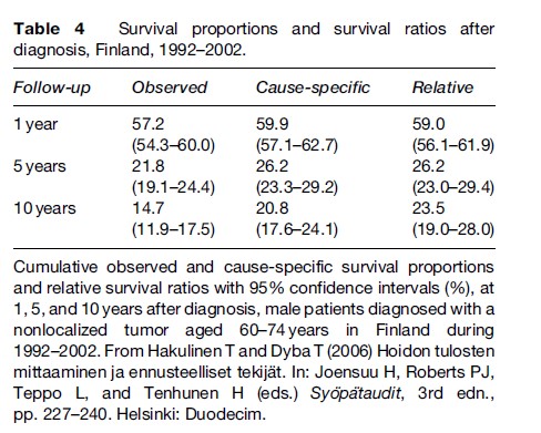
The survival proportion is an estimate of the probability of survival. A confidence interval expresses the range of values in which the true survival probability is most probably located. In a hypothetical repetition of 100 identical studies, the estimates from 95 studies would on average produce a 95% confidence interval covering the true value of the probability (provided that the statistical model used is appropriate). The confidence interval of the survival proportion (Table 4) is often based on a standard error obtained by Greenwood’s formula and an approximation based on the normal distribution.
For cause-specific survival, the numbers of deaths due to other causes are regarded as fixed. For relative survival, the expected survival is assumed to lack random error because it is usually based on the mortality experience of the (large) general population.
Differences between groups of patients in observed, cause-specific, and relative survival can be tested for statistical significance. The logrank test is most commonly used for observed and cause-specific survival, but it lacks power when the data are heavily grouped, e.g., with annual follow-up intervals. Alternatives with better power are available, which can also be used to test for differences in relative survival (Hakulinen et al., 1987).
Simple testing of the difference between survival proportions or ratios in observational studies is problematic, because the groups being compared were not formed by random allocation. The groups will usually differ with respect to many factors that should be controlled for in testing. This control in testing, including the logrank method and its extensions, is best done by proper statistical modeling (Dickman et al., 2004), which will be introduced in the section for regression analysis. Modeling both facilitates proper statistical testing and produces estimates that are adjusted for important prognostic factors.
The Maximally Updated Survival Estimates
The colon cancer patients in the example used here were diagnosed in Finland during 1992–2002 and followed up to the end of 2003. The problem with the survival estimates is that they tend to be outdated. For example, one can think that the 5-year survival analysis consists of a combination of five analyses, each specific to a follow-up year. The 1st-year analysis is based on follow-up that occurred in 1992–93 for those diagnosed in 1992, in 1993–94 for those diagnosed in 1993, and so on until in 2002–2003 for those diagnosed in 2002. A similar check reveals that also the 2nd-year, 3rd-year, etc., analyses are based on follow-up that occurred a longer time ago.
In demography, the current expectation of life is based on age-specific mortality rates of the most recent year. This principle can also be followed successfully in making an estimate for the current survival, based on the most recent 1st-year, 2nd-year, etc., follow-up year-specific figures. It is usual to use at least two recent calendar years, to avoid statistical uncertainty in the estimates arising from small numbers of events.
Many cancer registries use this period analysis (Brenner et al., 2004b) to produce maximally updated estimates of patient survival. For example in Finland, when all five follow-up year-specific analyses are based on follow-up that took place in 2001–2003, the 5-year relative survival for female colon cancer patients is 62%, whereas it is 59% based on the patients diagnosed during 1992–2002.
The period analysis result is based on patients who were followed up in 2001–2003. Patients diagnosed during 2000–2002 had their 1st year of follow-up within that time window 2001–2003 (no patients diagnosed in 2003 were included); patients diagnosed during 1999–2002 had their 2nd year of follow-up within that window, those diagnosed during 1998–2001 their 3rd year, etc., and those diagnosed during 1996–99 had their 5th year of follow-up within that time window.
In period analysis, both the period of diagnosis and that of the follow-up should be reported. Here, patients diagnosed during the period 1996–2002 and followed up during the period 2001–2003 were the basis of the analysis. Of these two periods, the period of follow-up, here 2001–2003, gives the name period analysis for 2001–2003 to the method.
Prognostic Factors
Prognostic factors can be divided into four groups: those related to the patient, the tumor, the diagnosis, and the treatment. Prognostic factors related to the patient include age, sex, symptoms, weight, genetic background, and immunological status. Tumor-related factors include tumor size, stage, histologic type, degree of malignancy, presence and location of metastases, hormone receptor status, and biochemical, molecular, and genetic markers. Diagnosis-related factors include the various diagnostic methods that may have been deployed and for solid tumors, the numbers of lymph nodes examined. Treatment-related factors also include the treatment techniques and their quality, e.g., dose intensity of cytostatic treatment and the total treatment time in radiation therapy.
All these factors may have independent effects on cancer survival, and they may also modify each other’s’ effects. The effects of certain factors may also be confounded by other factors. It may also depend on the context whether a certain effect should be regarded as confounding or not.
For example, one geographic region may have lower relative survival than another. Patients diagnosed in this region may have a less favorable distribution of disease stage. If diagnosing the tumors early has not been of high priority in that region and a comparison is made between the health system performances, it may be improper to adjust for stage, because stage is then a part of the outcome being studied, and thus an intervening variable on the causal pathway between the exposure under consideration (the performance of the health-care system) and the effect of that exposure (cancer-specific survival). On the other hand, it may only be of interest to compare cancer treatment services between the areas, and then adjustment for stage may be important. Thus, when survival comparisons are made between population groups, great care should be taken whether or not to adjust for the disease stage.
Population-based cancer registries normally collect information on a limited set of these variables, to enable monitoring of outcome over time and between population subgroups. In so-called high-resolution studies (Sant et al., 2003), this basic set of variables is extended, for representative samples of registered patients, by collection of additional data items from clinical and laboratory sources, e.g., diagnostic determinants or data on state-of-the-art treatment. This enables the explanatory impact of such variables on relative survival to be modeled.
Cause-Specific And Excess Mortality
With a large number of prognostic factors, estimating survival within each of the strata defined by the levels of those factors becomes difficult, because the required number of strata increases rapidly. The solution is statistical regression modeling of survival times, which can be based on individual data or on strata formed by individuals.
The most commonly used regression model is the Cox proportional hazards model, included in many software packages. It is possible and important to check and, when necessary, to give up the proportionality assumption in this method. This model can be used to study observed and cause-specific mortality. Observed (overall) mortality has two components, the first related to the cancer, the second due to other causes of death. It is unlikely that the second component would have the same prognostic factor background as the first.
In cause-specific analysis, only the first component of the overall risk of death is modeled. That is viable when the patients’ causes of death are available and can be assessed in a reliable and similar way in all the population subgroups to be compared and over time if the purpose of the study includes monitoring over time. Frequently, this ideal situation is not available. Death certification has changed over time and certification and coding practices have varied between countries and population subgroups to be compared. The solution is to model relative survival.
The Cox proportional hazards model has been generalized to relative survival. This allows relaxation of the assumption of proportionality, which does not usually hold in population-based data. In relative survival regression, the two components of mortality are explicitly recognized. The second component, the expected mortality, is estimated from life tables, and the difference between the total mortality and the expected mortality is then modeled. This difference, the excess mortality in the cancer patients, can generally be considered as attributable to the cancer. It may not always be true, for example if certain social classes or geographic areas are under or overrepresented among the cancer patients and this has not been taken into account in the selection of the general population comparison group, i.e., in the choice of life tables. For analyses comparing survival between social groups and geographic areas, it is particularly important to use the appropriate data on general mortality. Other factors such as smoking may make it difficult to identify a truly comparable general population group. For example, lung cancer patients tend to have a higher mortality due to many other smoking-related causes of death than just the lung cancer itself.
Finally, one might consider it important to exclude from the general population (or background) mortality that component of overall mortality that is due to the cancer being studied. This can be done, but the effect is generally small, because even the most common cancer typically accounts for only a small proportion of the total mortality in any one age group. For all cancers combined, however, it may be important if relative survival is to be used as an overall indicator of cancer survival when other causes of death have been eliminated. Such an analysis may be justified if relative survival is to be used as an index of the overall excess mortality of cancer patients.
Statistical modeling is based on the concept of hazard, the details of which will not be covered here. A mortality rate is an estimate of the hazard and for simplicity here it can be used synonymously. It is simply defined as the ratio between the number of deaths and the amount of persontime at risk.
Let us take the patients in Table 1 as an example. In the first interval, 62 deaths occurred. On the assumption that the deaths occurred, on average, in the middle of the interval, the patient group had n1 = 1230 – 62/2 = 1199 person-months at risk in that interval; there were no withdrawals (wi is zero). In general terms, the approximate formula for person-months at risk in interval i is ni = li – (di + wi)/2. The Finnish Cancer Registry data do not allow greater accuracy because the date of diagnosis does not include the day.
The observed mortality in the 1st month is thus 62/1199 person-months = 5.2/100 person-months or 62/100 person-years. Cause-specific mortality rates are 53/100 person-years for colon cancer and 9/100 person-years for other causes of death. In the section titled ‘Relative survival,’ it was noted that expected survival in each month of the 1st year was p1* = 0.9974, based on the corresponding general population mortality. This corresponds to an expected mortality of –ln[p1*] = 2.6/ 1000 person-months or 3.1/100 person-years (Dickman et al., 2004). In the 1st month, therefore, observed mortality among the cancer patients even due to causes of death other than cancer exceeds the expected mortality by almost threefold. Only nine such deaths were observed in that month, however, and after the 3rd month of followup, the numbers of deaths due to other causes are rather close to the expected number (Table 1). For example, in the 4th month of follow-up, the number of person-months at risk is n4 =1009 – 47/2 = 985.5, the expected mortality is 2.6/1000 person-months, as above, and so the expected number of deaths from other causes is 0.9855×2.6 = 2.56, close to the observed number of three deaths from other causes.
The excess mortality of the cancer patients is the difference between the total mortality rate and the expected mortality rate. In the first month in Table 1, it is 62/100 – 3.1/100 = 58.9/100 person-years. In the 4th month, the total mortality is 47/985.5 person-months or 57.2/100 person-years and the excess mortality thus 57.2/ 100 – 3.1/100 = 54.1/100 person-years, slightly lower than in the 1st month.
Regression Analyses
Regression analysis with the Cox proportional hazards model and its extension for relative survival (Dickman et al., 2004) can be conducted with statistical software packages such as SAS, STATA, R and S+. Let us now look at modeling the cause-specific and relative survival during the first 5 years of follow-up for the patients in Table 3.
The results (Table 5) show the ratios between the cause-specific mortality rates (cause-specific hazard ratios) in different age groups and time intervals since diagnosis, and, similarly, ratios between the excess mortality rates (excess hazard ratios). For example, the cause-specific hazard ratio for women is 0.95 that of men (reference) and the excess mortality hazard ratio is 0.93, i.e. women have a 5–7% advantage over the males. According to this model, the advantage holds true for the 5 years of follow-up. The hazard ratios are significantly lower by 15–17% for patients diagnosed during 1998–2002 than for those diagnosed during 1992–97.
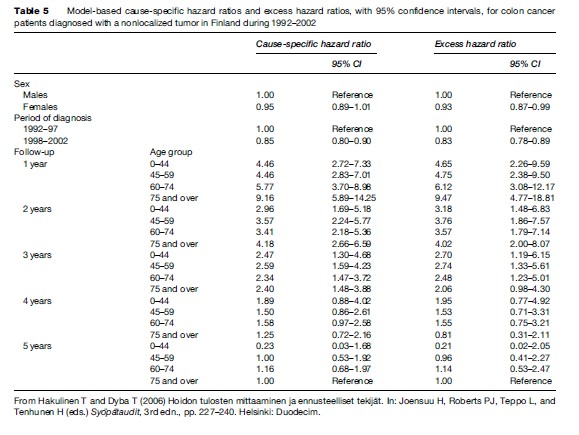
The models for cause-specific and relative survival both introduce an interaction between age and time since diagnosis, meaning that the cause-specific and excess hazards do not retain their proportionality between age groups throughout the duration of follow-up. The differences in the hazard between the age groups are the largest in the first interval and nearly disappear by the third interval. Methods exist to smooth these effects and to provide a continuous representation for the interaction (Remontet et al., 2007).
It is important that the analysis does not stop after the coefficients of Table 5 have been obtained. When the model adequately describes the data, model-based estimates with standard errors should be calculated for the cause-specific survival proportions and the relative survival ratios. The model-based estimates have smaller standard errors than the empirical estimates, because the entire data set has been used in the model, rather than a particular subset (Table 6). The modeling has thus removed unnecessary randomness from the estimates.

In principle, the modeled results are also free from problems caused by differences in potential follow-up times by age group. The validity of the independence assumption between the causes of death can be improved by a finer stratification by age.
Proportion Cured, Parametric Methods
It was roughly estimated from Figure 4 that the point of cure for Finnish colon cancer patients diagnosed in 1992–2002 was achieved after approximately 9 years of follow-up. Thus the proportion cured is practically the same as the 10-year cumulative relative survival by sex and age (Table 3).
It is possible to study cure systematically by fitting parametric excess mortality models that explicitly include the possibility of cure for a proportion of patients (De Angelis et al., 1999), and that the proportion cured may depend on prognostic factors. The cured patients are considered as subject to general population mortality only, i.e., having no excess mortality. The proportion of patients who are not cured (fatal cases), or those bound to die from their cancer in the absence of competing risks of death, may be characterized by the mean or median duration of survival.
The proportion cured and the mean duration of survival for fatal cases have both increased for Finnish colon cancer patients. For males aged 65–74 years at diagnosis, some 20% of those diagnosed during 1953–59 were cured, whereas the proportion rose to 44% for those diagnosed during 1980–92. At the same time, the mean survival time for fatal cases increased from 0.59 to 1.51 years. Earlier diagnosis and more effective treatment may both be involved in these favorable trends.
Summarizing Results, Age Standardization
The results in Tables 5 and 6 can conveniently be used to summarize survival trends over time and differences between populations. However, there is still a need for conventional methods as for direct standardization, particularly if model-based results are not available. Model-based results may also be standardized for age, particularly when the empirical stratum-specific results have large standard errors and are thus very inaccurately estimated.
The standardization of survival proportions and particularly of relative survival ratios is much more complicated than that for incidence rates, because of the follow-up time dimension. The choice of method depends on the desired interpretation of the standardized ratio.
The traditional interpretation of a directly age standardized survival proportion is the survival that would be observed in the index population of cancer patients under study if its age structure were the same as that in a chosen standard population. The solution is to stratify the analysis by age and to take a weighted average of the age-specific survival curves as the age-standardized survival curve.
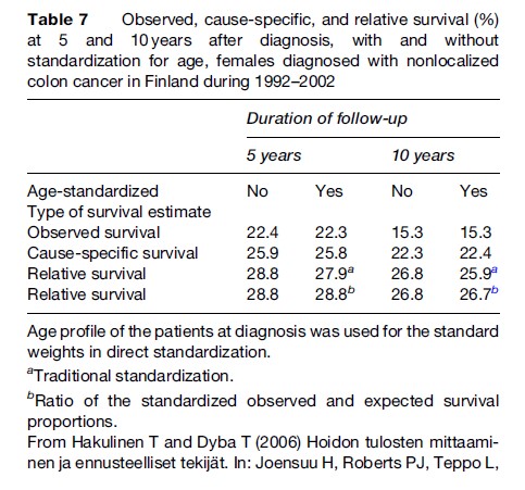
For example, due to demographic changes the number of old patients can increase by calendar time, whereas that of young patients does not. As a consequence, the old patients have, on average, shorter potential follow-up times than the young patients, and the more favorable survival of the young patients that can be followed longer will be predicted for the old patients after the time of censoring. The result is that the nonstandardized survival proportions will be higher than the age-standardized proportions even when the age distribution of the patients themselves is used as a standard. This is not a problem for colon cancer patients diagnosed in Finland in 1992–2002 (Table 7).
Two new methods of age standardization have been proposed by Brenner and Hakulinen (2003) and Brenner et al. (2004a). They both use time-varying weights and the newer of them does not presuppose any age stratification, which is very advantageous with smaller data sets. They are both consistent with the interpretation of relative survival as a ratio and not an estimate of cancer-specific survival probability.
Traditional standardization is required at least in longer-term follow-up for probability interpretation of the relative survival ratio even when there is no aim at comparisons between populations. Standardization controls both the effect of informative censoring and that of dependence between the causes of death. Standardization may also be needed for comparisons between patient populations, even when the age structures of the populations do not differ when there is informative censoring by age.
With the exception of one standardization method for the ratio interpretation of the relative survival ratio (Brenner et al., 2004a), all the age standardization methods presented depend on survival analyses stratified by age.
There are three different methods for calculation of the expected survival, and hence for the relative survival ratio, two proposed by Ederer et al. (1959, 1961) and one proposed by Hakulinen (1982). With stratified analyses, such as age standardization with the direct method, and nonstratified analyses up to 10 years of follow-up, it does not in practice matter which one of the methods is used. In longer-term follow-up for nonstratified and nonstandardized analyses, as well as in the standardization method of Brenner et al. (2004a), the method proposed by Hakulinen should be used because it gives the best control against informative censoring.
Concluding Practical Remarks
The relative survival ratio was proposed in 1950 by Berkson and Gage (Berkson and Gage, 1950). Ever since then, it has been used to monitor progress in population-based cancer survival, in the United States (the SEER project), in Europe (the EUROCARE project), in the world (the CONCORD project), and in many countries and cancer registration areas.
Socioeconomic differences generally determine the differences observed. Thus, for example, differences in relative survival could directly be related to the degree of deprivation of the population in England and Wales (Coleman et al., 1999), whereas differences within the Nordic countries by region and in Finland by social class were small (Dickman et al., 1997). Diagnostic determinants, e.g., numbers of lymph nodes examined, explain differences observed in relative survival between European countries and between Europe and the United States. Comparability of disease definition is still an issue in attempts to further elucidate the advantage that American patients tend to have in relative survival compared to European patients. To aid in the interpretation of relative survival, it is useful to examine the corresponding incidence and mortality rates (Dickman and Adami, 2006).
Estimates of relative survival do not depend on the certified cause of death, or on temporal trends or socio-geographic differences in death certification practices. This property of relative survival is extremely valuable for examining trends or differences in survival, in direct contrast with cause-specific survival proportions. In Finland, where death certification is accurate and where the cancer registry uses causes of death that, when necessary, have been corrected by the registry, relative and cause-specific survival analyses quite often give results that agree with each other. This provides further empirical support to the validity of relative survival as an estimate of cause-specific survival.
Nevertheless, interpretation of relative survival requires care. The general population group must be comparable with the patient group, particularly for analyses specific to region, social class, or degree of deprivation (Dickman et al., 1998).
Tumors are increasingly diagnosed early. As a result, survival times become longer even when there is no true improvement in the sense of postponement of death. Screening or particularly intense diagnostic activity, especially with prostatic cancer, may also lead to the diagnoses of cases that would not otherwise have been detected during the person’s lifetime. These cases, naturally, have favorable survival.
The methods of tumor diagnosis have changed over time. Consider the spectrum of disease progression in just two categories, localized and nonlocalized. In the past, when diagnostic facilities were less effective at detecting metastatic spread than they are now, cases described as localized would have included some that would now be classified, more correctly, as nonlocalized. As a result, newly diagnosed cases described as localized are now, on average, even less advanced than in the past. Similarly, nonlocalized cases now include some that are less advanced, and on average, nonlocalized cases are also less advanced than in the past. This was reflected in trends of survival from cancer of the oral cavity in females in Finland over the period 1953–74: Relative survival increased with time both for localized and for nonlocalized cases, whereas for all cases combined, there was no change (Hakulinen, 1983). This problem, called stage migration, does not just apply over time; it also affects stage-specific comparisons between populations.
Newly diagnosed patients included in cancer registries normally include a small proportion of cases for whom the diagnosis is based solely on a death certificate or autopsy. These cases are often excluded from survival analyses because the diagnosis is based on persons who are already dead, and for whom the date of diagnosis (and thus the duration of survival) is unknown. Some cancer registries, more than others, try to trace back the individuals of whom the first notification came through a death certificate. Sometimes this is successful. On average, these so-called death-certificate-initiated cases have poorer survival than the other patients. Thus, attempts to trace back (or follow-back) individuals may confer the cancer registry area a somewhat lower patient survival compared with another area where follow-back is not done.
On the other hand, a large proportion of cases in the cancer registry’s database with diagnosis based solely on a death certificate or autopsy is likely to be an indication that the registry may miss the recording of many nonfatal cases. This leads to survival that is unduly low. This has been one of the possible explanations behind the observation that the relative survival in England and Wales tends to be lower than in the other countries of Western Europe.
A high proportion of cases in which there is microscopic confirmation of the diagnosis is also important for unbiased survival analysis. If survival is high for patients with a cancer that is usually fatal, this may indicate poor quality of diagnostic information.
High survival figures are also observed when there are problems in the follow-up of patients. Relative survival is again a very good indicator of data quality: If relative survival ratios within successive intervals show that patients survive more favorably in the long term than the general population, there is reason to suspect incompleteness of the cancer registry’s follow-up procedures to ascertain the deaths of registered patients.
Population-based relative survival is a challenging concept to use. It can be used for many important purposes within cancer control, and its use has certainly led to changes in public health policy to improve the diagnosis, treatment, and care of cancer patients. But the use of relative survival requires considerable care and a sound understanding of the basic data, as well as of the underlying principles and methods.
Bibliography:
- Berkson J and Gage RP (1950) Calculation of survival rates for cancer. Proceedings of Staff Meetings of the Mayo Clinic 25: 270–286.
- Berrino F, Capocaccia R Coleman MP, et al. (eds.) (2003) Survival of Cancer Patients in Europe: the EUROCARE-3 study. Annals of Oncology 14(supplement 5): 1–155.
- Brenner H and Hakulinen T (2003) On crude and age-adjusted relative survival rates. Journal of Clinical Epidemiology 56: 1185–1191.
- Brenner H, Arndt V, Gefeller O, and Hakulinen T (2004a) An alternative approach to age adjustment of cancer survival rates. European Journal of Cancer 40: 2317–2322.
- Brenner H, Gefeller O, and Hakulinen T (2004b) Period analysis for ‘‘up-to-date’’ cancer survival data: Theory, empirical evaluation, computational realisation and applications. European Journal Cancer 40: 326–335.
- Coleman MP, Babb P, Damiecki P, et al. (1999) Cancer Survival Trends in England and Wales 1971–1995: Deprivation and NHS Region. London: The Stationery Office.
- DeAngelis R, Capocaccia R, Hakulinen T, So¨ derman B, and Verdecchia A (1999) Mixture models for cancer survival analysis: Application to population-based data with covariates. Statistics in Medicine 18: 441–454.
- Dickman P and Adami H-O (2006) Interpreting trends in cancer patient survival. Journal of Internal Medicine 260: 103–117.
- Dickman PW, Gibberd RW, and Hakulinen T (1997) Estimating potential savings in cancer deaths by eliminating regional and social class variation in cancer survival in the Nordic countries. Journal of Epidemiology and Community Health 51: 289–298.
- Dickman PW, Auvinen A, Voutilainen ET, and Hakulinen T (1998) Measuring social class differences in cancer patient survival: Is it necessary to control for social class differences in general population mortality? A Finnish population-based study. Journal of Epidemiology and Community Health 52: 1–8.
- Dickman PW, Sloggett A, Hills M, and Hakulinen T (2004) Regression models for relative survival. Statistics in Medicine 23: 51–64.
- Ederer F and Heise H (1959) Instructions to IBM 650 Programmes in Processing Survival Computations. Methodological Note No. 10. Bethesda, MD: End Results Evaluation Section. National Cancer Institute.
- Ederer F, Axtell LM, and Cutter SJ (1961) The Relative Survival Rate: A Statistical Methodology. UICC Technical Report Series. pp. 101–121. Bethesda, MD: National Cancer Institute
- Elandt-Johnson RC (1975) Definition of rates: Some remarks on their use and misuse. American Journal of Epidemiology 102: 267–271.
- Hakulinen T (1982) Cancer survival corrected for heterogeneity in patient withdrawal. Biometrics 38: 933–942.
- Hakulinen T (1983) A comparison of nationwide cancer survival statistics in Finland and Norway. World Health Statistics Quarterly 36: 35–46.
- Hakulinen T and Dyba T (2006) Hoidon tulosten mittaaminen ja ennusteelliset tekija¨ t. In: Joensuu H, Roberts PJ, Teppo L, and Tenhunen H (eds.) Syo¨pa¨taudit, 3rd edn., pp. 227–240. Helsinki Finland: Duodecim.
- Hakulinen T, Tenkanen L, Abeywickrama K, and Pa¨ iva¨ rinta L (1987) Testing equality of relative survival patterns based on aggregated data. Biometrics 43: 313–325.
- Remontet L, Bossard N, Belot A, Este` ve J and the French Network of Cancer Registries FRANCIM (2007) An overall strategy based on regression models to estimate relative survival and model the effects of prognostic factors in cancer survival studies. Statistics in Medicine 26: 2214–2228.
- Sant M, Allemani C, Capocaccia R, et al. (2003) Stage at diagnosis is a key explanation of differences in breast cancer survival across Europe. International Journal of Cancer 106: 416–422; 107: 1058 (erratum).
- Brenner H and Hakulinen T (2006) Up-to-date and precise estimates of cancer patient survival: Model-based period analysis. American Journal of Epidemiology 164: 689–696.
- Hakama M and Hakulinen T (1977) Estimating the expectation of life in cancer survival studies with incomplete follow-up information. Journal of Chronic Diseases 30: 585–597.
- Hakulinen T (1977) On long-term relative survival rates. Journal of Chronic Diseases 30: 431–443.
- Heina¨ vaara S, Teppo L, and Hakulinen T (2002) Cancer-specific survival of patients with multiple cancers: An application to patients with multiple breast cancers. Statistics in Medicine 21: 3183–3195.
- Parkin DM and Hakulinen T (1991) Analysis of survival. In: Jensen OM, Parkin DM, MacLennan R, Muir CS, and Skeet RG (eds.) Cancer Registration: Principles and Methods. IARC Scientific Publications No 95. pp. 159–176. Lyon, France: International Agency for Research on Cancer.
- Verdecchia A, DeAngelis G, and Capocaccia R (2002) Estimation and projections of cancer prevalence from cancer registry data. Statistics in Medicine 21: 3511–3526.
- http://www.eurocare.it/ – EUROCARE, Survival of cancer patients in Europe.
- http://unimed.mf.uni-lj.si/relsurv/index.pl – European Information Network-Ethics in Medicine and Biotechnology, Calculate your individual relative survival.
- https://seer.cancer.gov/ – National Cancer Institute, Surveillance, Epidemiology and End Results.


